Visualize cells and gene expression according to spatial coordinates
spatGenePlot2D(
  gobject,
  show_image = F,
  gimage = NULL,
  image_name = "image",
  sdimx = "sdimx",
  sdimy = "sdimy",
  expression_values = c("normalized", "scaled", "custom"),
  genes,
  cell_color_gradient = c("blue", "white", "red"),
  gradient_midpoint = NULL,
  gradient_limits = NULL,
  show_network = F,
  network_color = NULL,
  spatial_network_name = "Delaunay_network",
  edge_alpha = NULL,
  show_grid = F,
  grid_color = NULL,
  spatial_grid_name = "spatial_grid",
  midpoint = 0,
  scale_alpha_with_expression = FALSE,
  point_shape = c("border", "no_border", "voronoi"),
  point_size = 1,
  point_alpha = 1,
  point_border_col = "black",
  point_border_stroke = 0.1,
  show_legend = T,
  legend_text = 8,
  background_color = "white",
  vor_border_color = "white",
  vor_alpha = 1,
  vor_max_radius = 200,
  axis_text = 8,
  axis_title = 8,
  cow_n_col = 2,
  cow_rel_h = 1,
  cow_rel_w = 1,
  cow_align = "h",
  show_plot = NA,
  return_plot = NA,
  save_plot = NA,
  save_param = list(),
  default_save_name = "spatGenePlot2D"
)
Arguments
| gobject | giotto object |
|---|---|
| show_image | show a tissue background image |
| gimage | a giotto image |
| image_name | name of a giotto image |
| sdimx | x-axis dimension name (default = 'sdimx') |
| sdimy | y-axis dimension name (default = 'sdimy') |
| expression_values | gene expression values to use |
| genes | genes to show |
| cell_color_gradient | vector with 3 colors for numeric data |
| gradient_midpoint | midpoint for color gradient |
| gradient_limits | vector with lower and upper limits |
| show_network | show underlying spatial network |
| network_color | color of spatial network |
| spatial_network_name | name of spatial network to use |
| edge_alpha | alpha of edge |
| show_grid | show spatial grid |
| grid_color | color of spatial grid |
| spatial_grid_name | name of spatial grid to use |
| midpoint | expression midpoint |
| scale_alpha_with_expression | scale expression with ggplot alpha parameter |
| point_shape | shape of points (border, no_border or voronoi) |
| point_size | size of point (cell) |
| point_alpha | transparancy of points |
| point_border_col | color of border around points |
| point_border_stroke | stroke size of border around points |
| show_legend | show legend |
| legend_text | size of legend text |
| background_color | color of plot background |
| vor_border_color | border colorr for voronoi plot |
| vor_alpha | transparancy of voronoi 'cells' |
| vor_max_radius | maximum radius for voronoi 'cells' |
| axis_text | size of axis text |
| axis_title | size of axis title |
| cow_n_col | cowplot param: how many columns |
| cow_rel_h | cowplot param: relative height |
| cow_rel_w | cowplot param: relative width |
| cow_align | cowplot param: how to align |
| show_plot | show plots |
| return_plot | return ggplot object |
| save_plot | directly save the plot [boolean] |
| save_param | list of saving parameters, see |
| default_save_name | default save name for saving, don't change, change save_name in save_param |
Value
ggplot
Details
Description of parameters.
See also
Other spatial gene expression visualizations:
spatGenePlot3D(),
spatGenePlot()
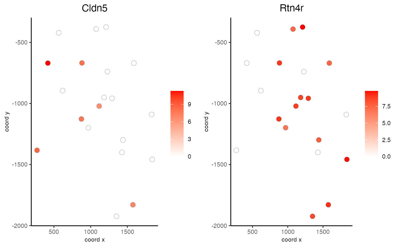
Examples
data(mini_giotto_single_cell)

all_genes = slot(mini_giotto_single_cell, 'gene_ID')
selected_genes = all_genes[1:2]
spatGenePlot2D(mini_giotto_single_cell, genes = selected_genes, point_size = 3)