#> Warning: This tutorial was written with Giotto version 0.3.6.9046, your version
#> is 1.0.3.This is a more recent version and results should be reproduciblelibrary(Giotto) # 1. set working directory results_folder = '/path/to/directory/' # 2. set giotto python path # set python path to your preferred python version path # set python path to NULL if you want to automatically install (only the 1st time) and use the giotto miniconda environment python_path = NULL if(is.null(python_path)) { installGiottoEnvironment() }
Dataset explanation
10X genomics recently launched a new platform to obtain spatial expression data using a Visium Spatial Gene Expression slide.
The Visium brain data to run this tutorial can be found here
Visium technology: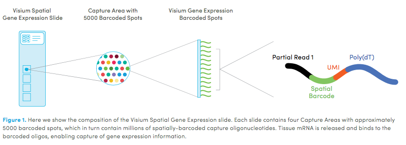
High resolution png from original tissue: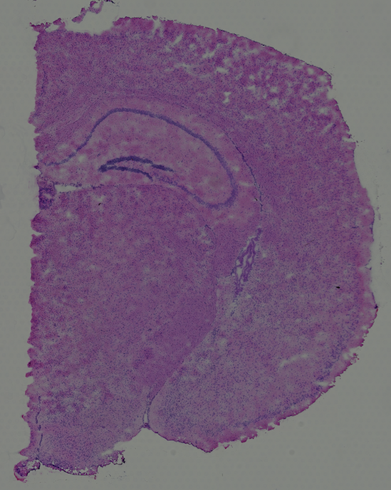
Part 1: Giotto global instructions and preparations
## create instructions
instrs = createGiottoInstructions(save_dir = results_folder,
                                  save_plot = TRUE,
                                  show_plot = FALSE)

## provide path to visium folder
data_path = '/path/to/Brain_data/'
part 2: Create Giotto object & process data
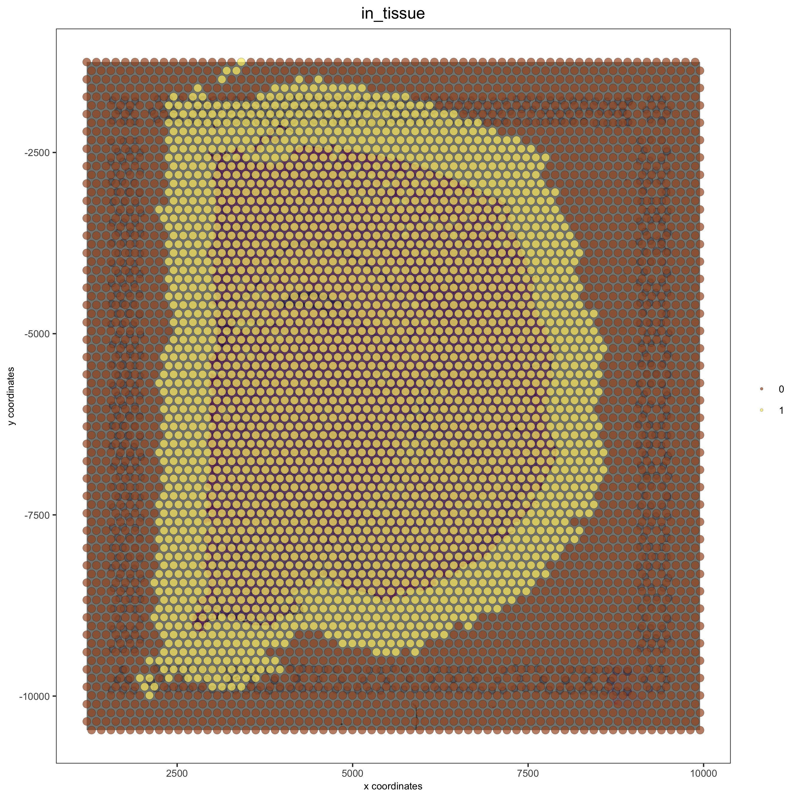
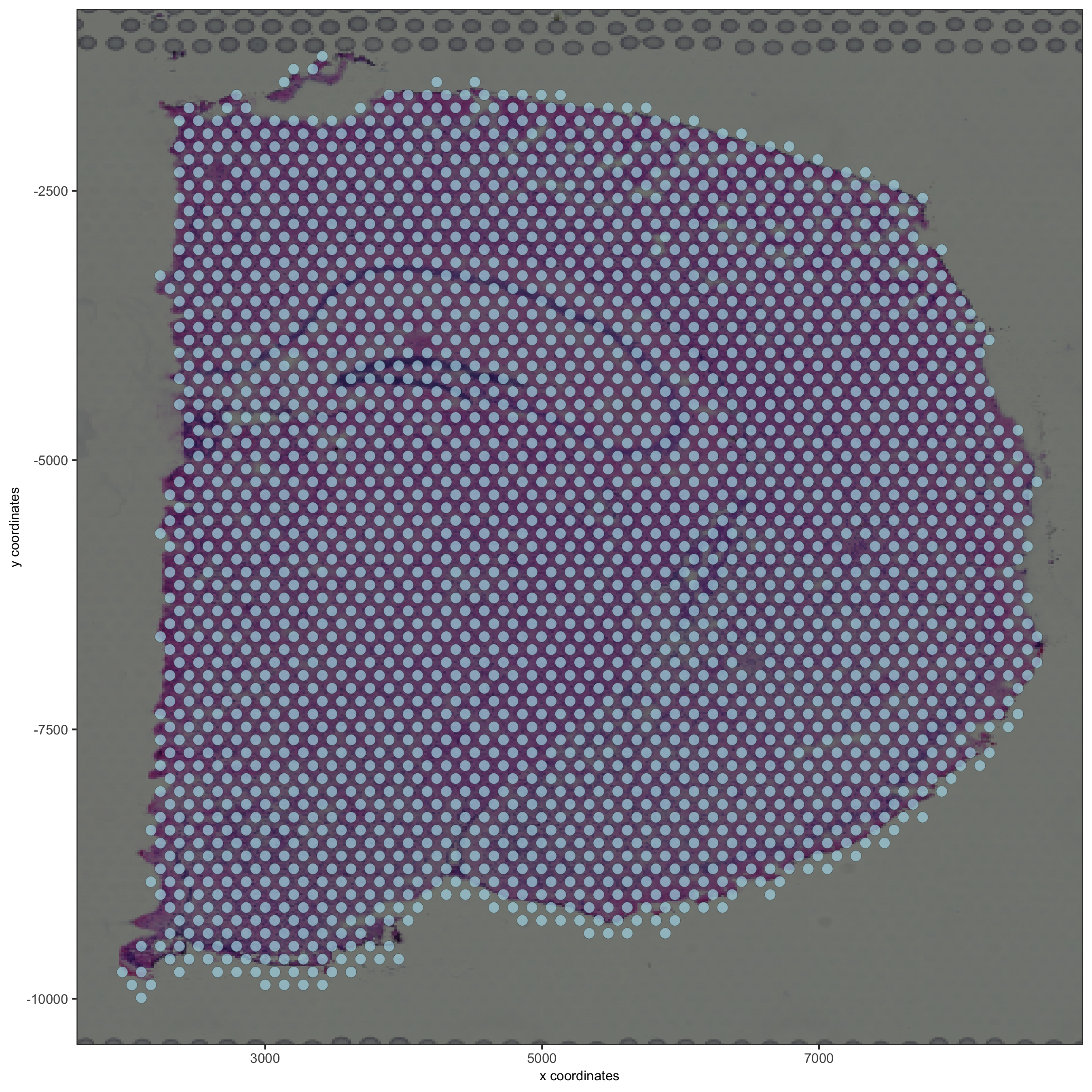
## directly from visium folder
visium_brain = createGiottoVisiumObject(visium_dir = data_path, expr_data = 'raw',
                                         png_name = 'tissue_lowres_image.png',
                                         gene_column_index = 2, instructions = instrs)

## update and align background image
# problem: image is not perfectly aligned
spatPlot(gobject = visium_brain, cell_color = 'in_tissue', show_image = T, point_alpha = 0.7,
         save_param = list(save_name = '2_a_spatplot_image'))
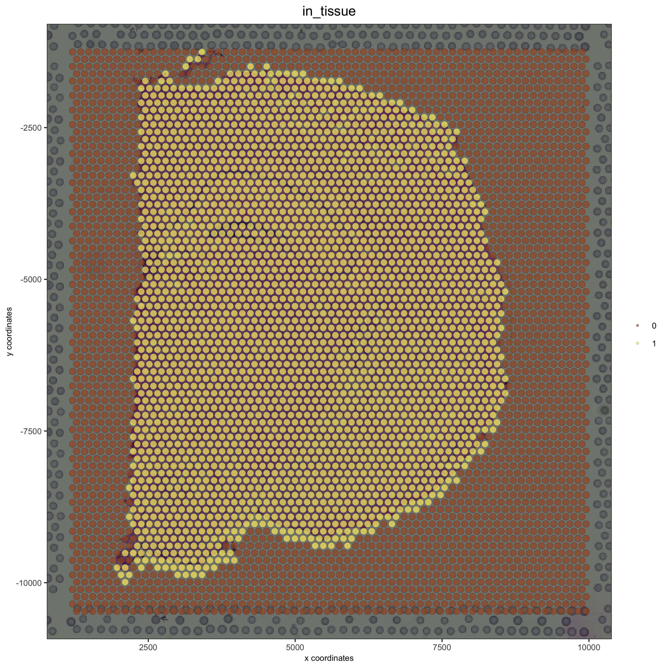
# check name
showGiottoImageNames(visium_brain) # "image" is the default name
# adjust parameters to align image (iterative approach)
visium_brain = updateGiottoImage(visium_brain, image_name = 'image',
                                  xmax_adj = 1300, xmin_adj = 1200,
                                  ymax_adj = 1100, ymin_adj = 1000)

# now it's aligned
spatPlot(gobject = visium_brain, cell_color = 'in_tissue', show_image = T, point_alpha = 0.7,
         save_param = list(save_name = '2_b_spatplot_image_adjusted'))
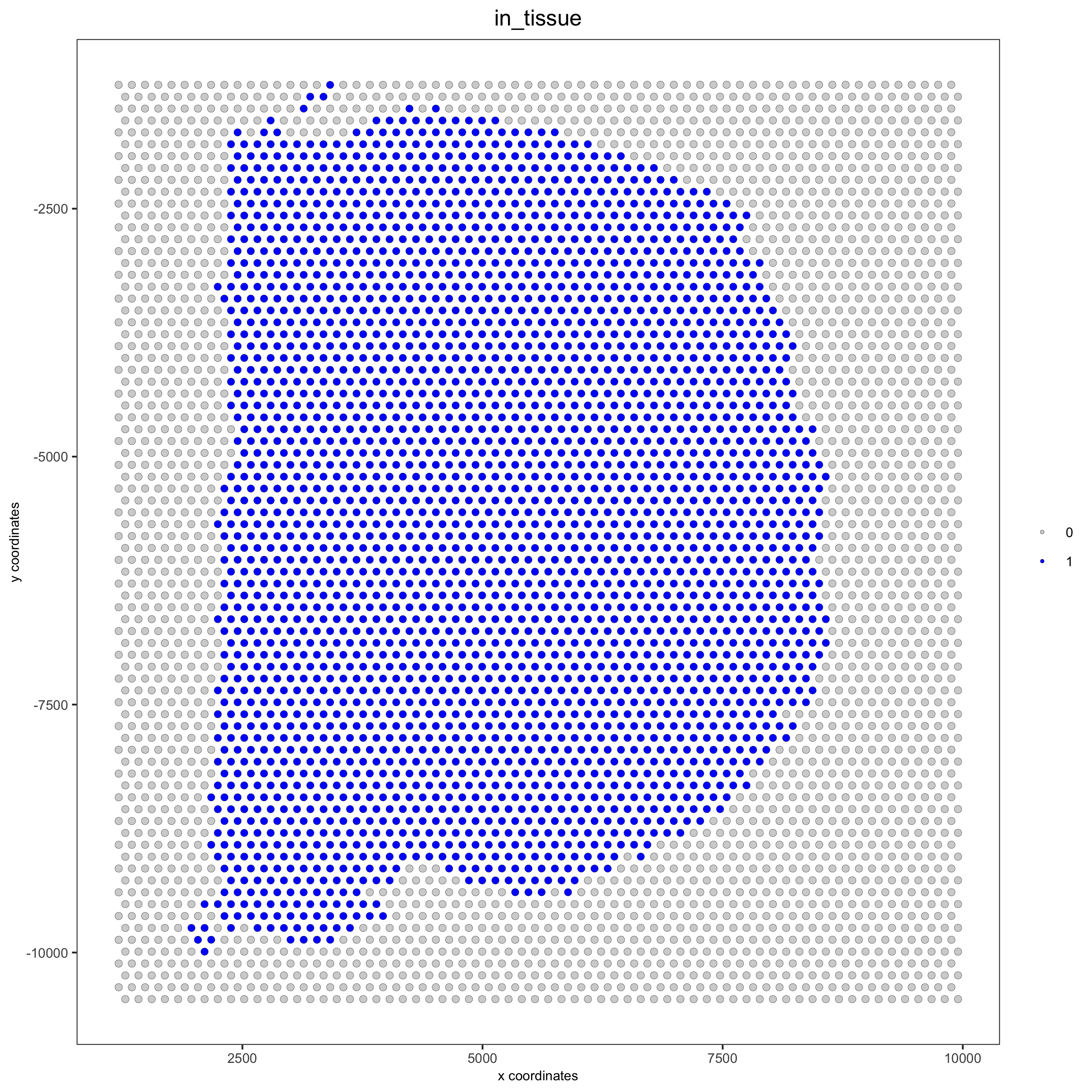
## check metadata
pDataDT(visium_brain)

## compare in tissue with provided jpg
spatPlot(gobject = visium_brain, cell_color = 'in_tissue', point_size = 2,
         cell_color_code = c('0' = 'lightgrey', '1' = 'blue'),
         save_param = list(save_name = '2_c_in_tissue'))
## subset on spots that were covered by tissue
metadata = pDataDT(visium_brain)
in_tissue_barcodes = metadata[in_tissue == 1]$cell_ID
visium_brain = subsetGiotto(visium_brain, cell_ids = in_tissue_barcodes)

## filter
visium_brain <- filterGiotto(gobject = visium_brain,
                              expression_threshold = 1,
                              gene_det_in_min_cells = 50,
                              min_det_genes_per_cell = 1000,
                              expression_values = c('raw'),
                              verbose = T)

## normalize
visium_brain <- normalizeGiotto(gobject = visium_brain, scalefactor = 6000, verbose = T)

## add gene & cell statistics
visium_brain <- addStatistics(gobject = visium_brain)

## visualize
spatPlot2D(gobject = visium_brain, show_image = T, point_alpha = 0.7,
           save_param = list(save_name = '2_d_spatial_locations'))
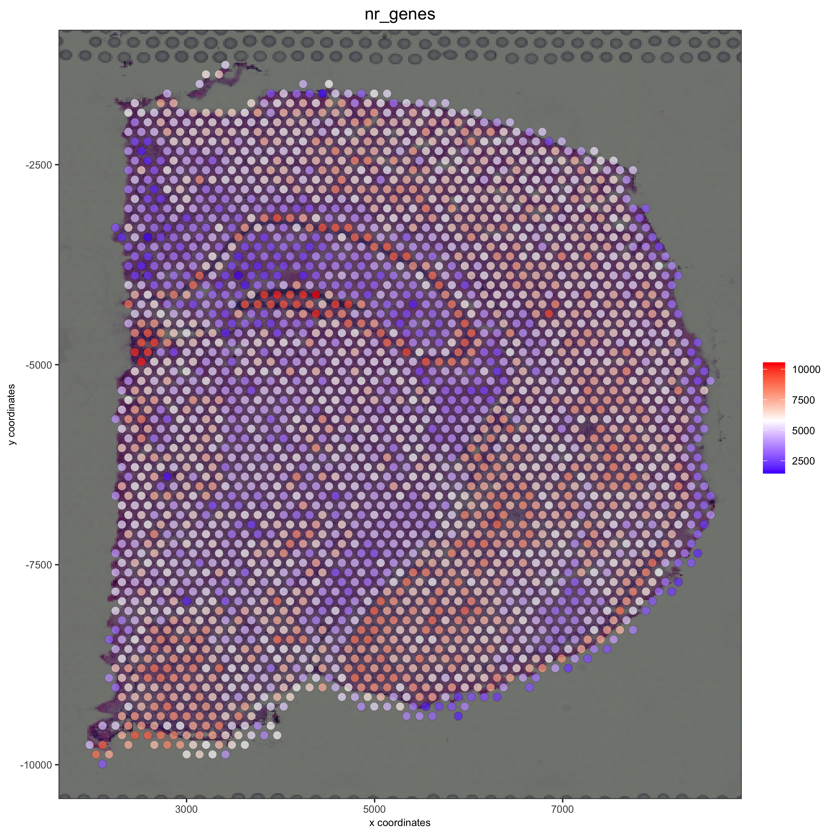
spatPlot2D(gobject = visium_brain, show_image = T, point_alpha = 0.7,
           cell_color = 'nr_genes', color_as_factor = F,
           save_param = list(save_name = '2_e_nr_genes'))
part 3: dimension reduction
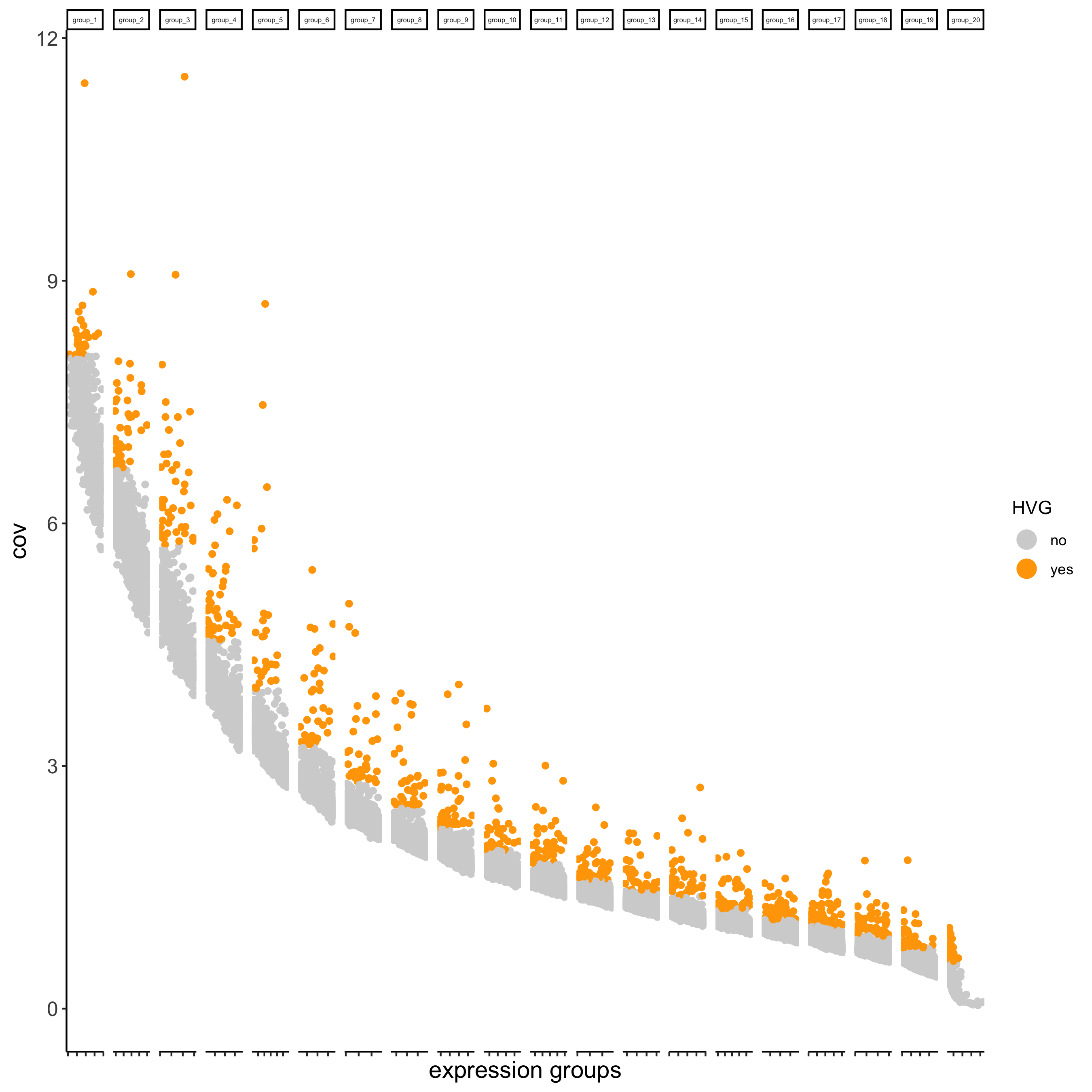
## highly variable genes (HVG)
visium_brain <- calculateHVG(gobject = visium_brain,
                              save_param = list(save_name = '3_a_HVGplot'))
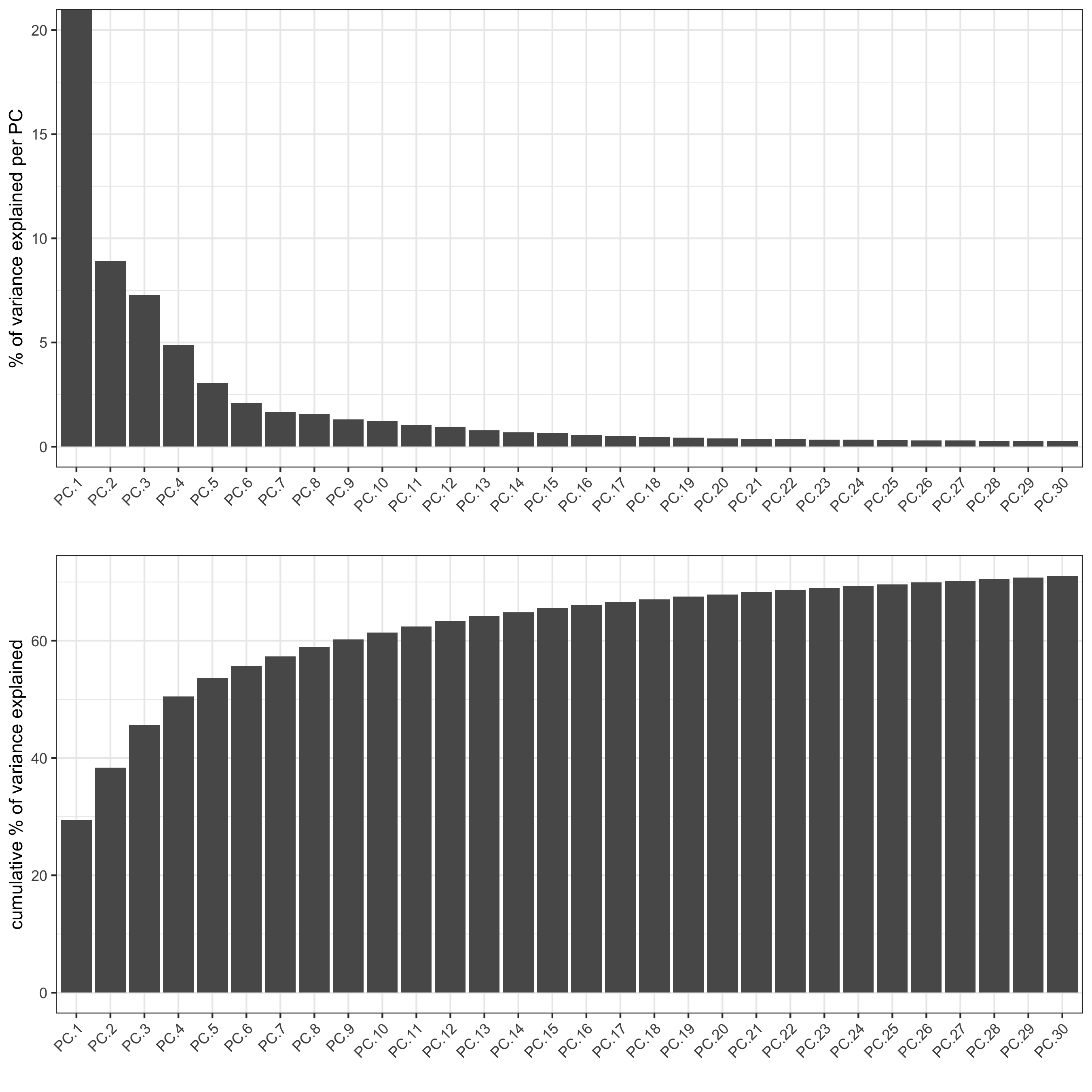
## run PCA on expression values (default)
gene_metadata = fDataDT(visium_brain)
featgenes = gene_metadata[hvg == 'yes' & perc_cells > 3 & mean_expr_det > 0.4]$gene_ID

visium_brain <- runPCA(gobject = visium_brain,
                       genes_to_use = featgenes,
                       scale_unit = F, center = T,
                       method="factominer")

screePlot(visium_brain, ncp = 30, save_param = list(save_name = '3_b_screeplot'))
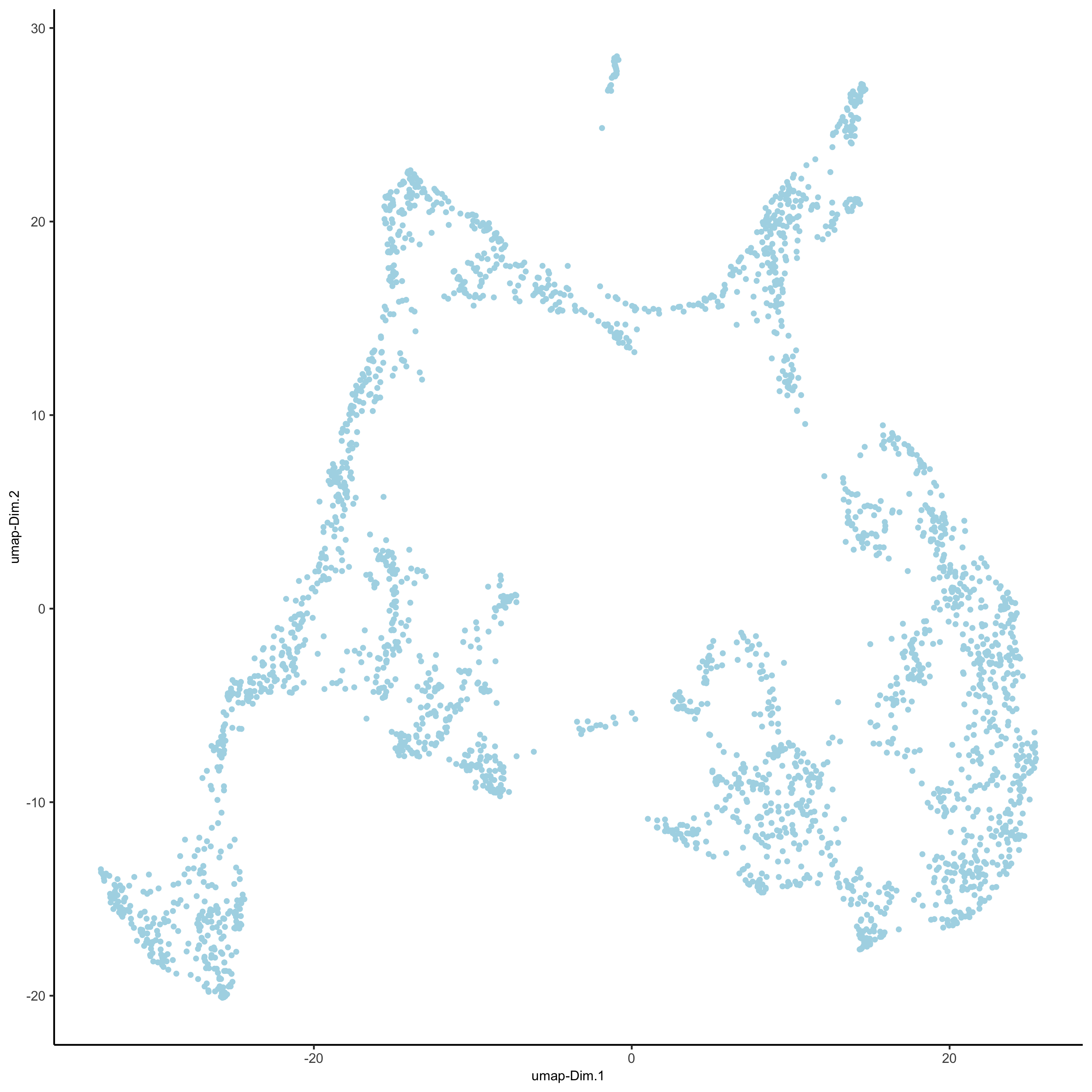
## run UMAP and tSNE on PCA space (default)
visium_brain <- runUMAP(visium_brain, dimensions_to_use = 1:10)
plotUMAP(gobject = visium_brain,
         save_param = list(save_name = '3_d_UMAP_reduction'))
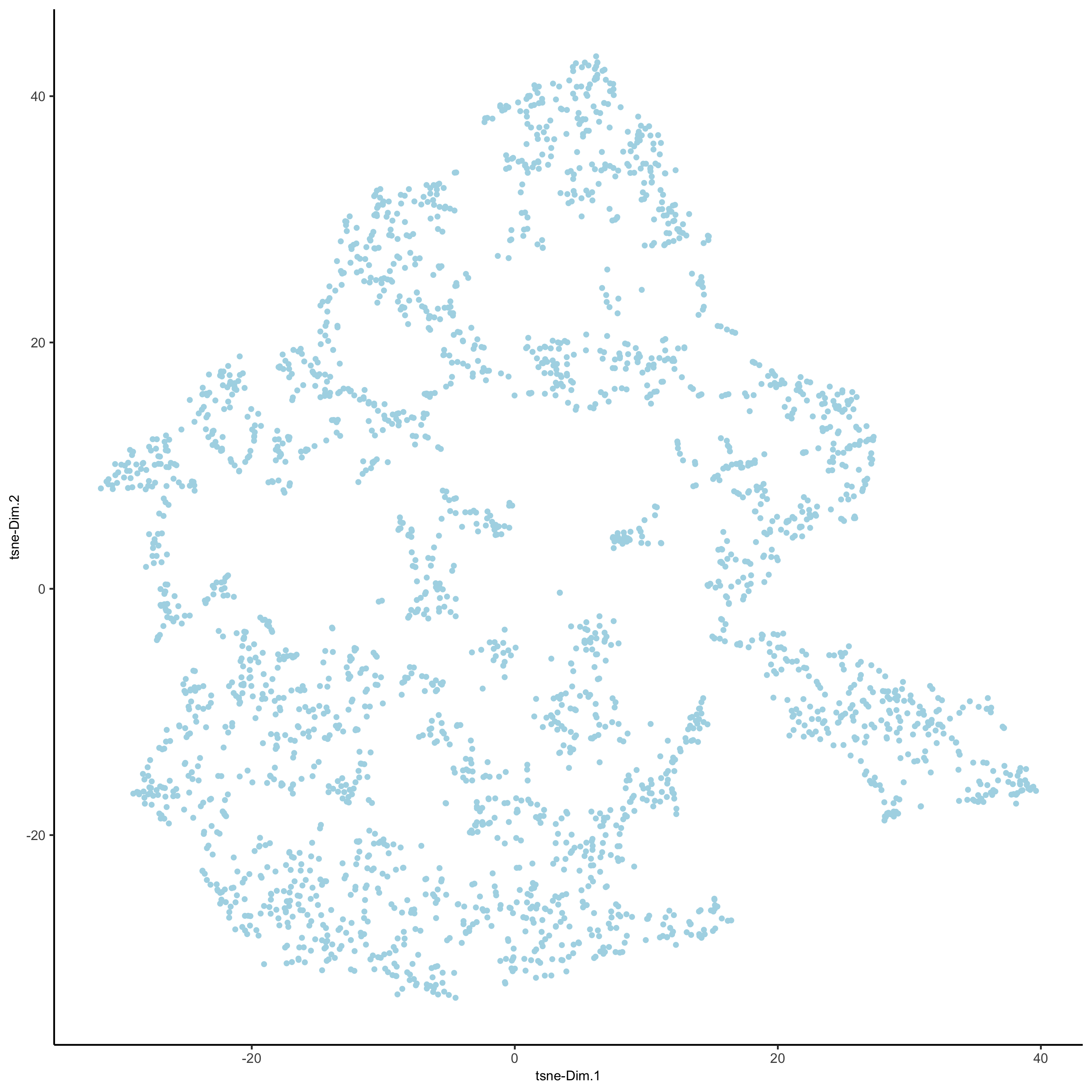
visium_brain <- runtSNE(visium_brain, dimensions_to_use = 1:10)
plotTSNE(gobject = visium_brain,
         save_param = list(save_name = '3_e_tSNE_reduction'))
part 4: cluster
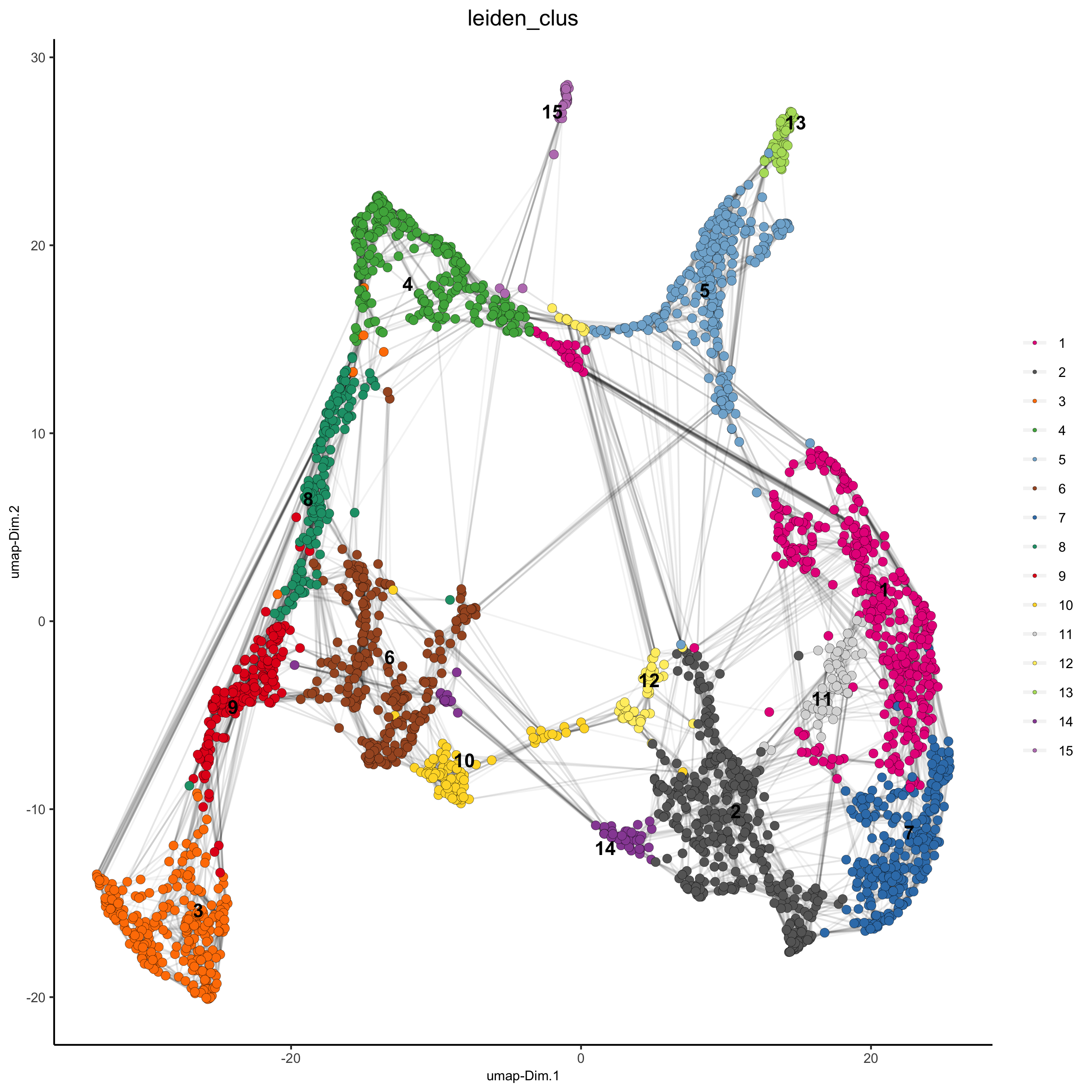
## sNN network (default)
visium_brain <- createNearestNetwork(gobject = visium_brain, dimensions_to_use = 1:10, k = 15)
## Leiden clustering
visium_brain <- doLeidenCluster(gobject = visium_brain, resolution = 0.4, n_iterations = 1000)
plotUMAP(gobject = visium_brain,
         cell_color = 'leiden_clus', show_NN_network = T, point_size = 2.5,
         save_param = list(save_name = '4_a_UMAP_leiden'))
part 5: co-visualize
5.1 whole dataset
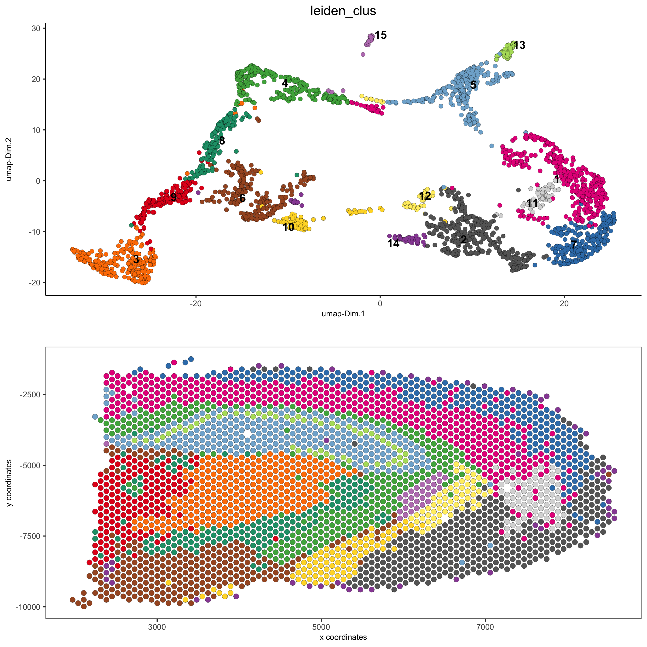
# expression and spatial
spatDimPlot(gobject = visium_brain, cell_color = 'leiden_clus',
            dim_point_size = 2, spat_point_size = 2.5,
            save_param = list(save_name = '5_a_covis_leiden'))
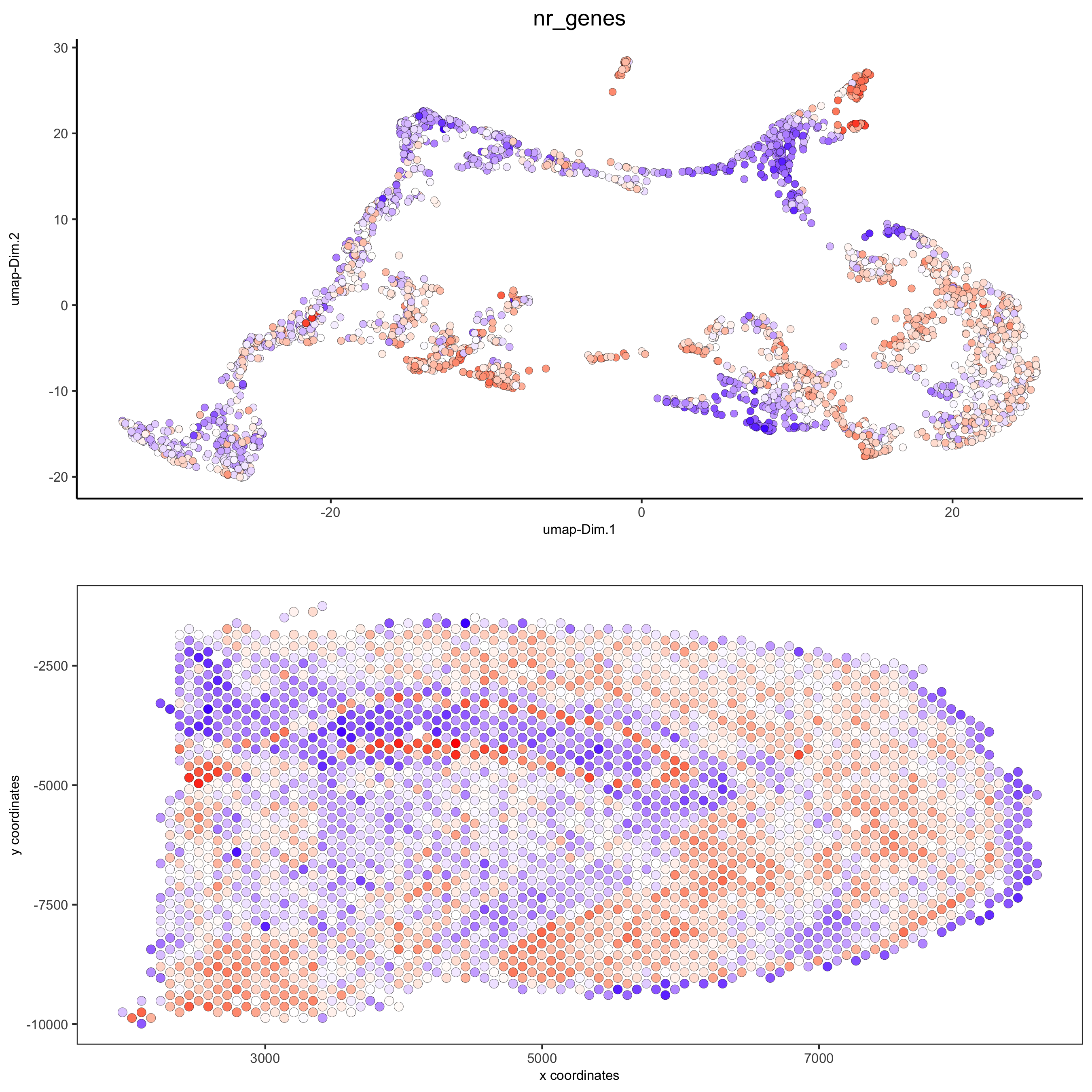
spatDimPlot(gobject = visium_brain, cell_color = 'nr_genes', color_as_factor = F,
            dim_point_size = 2, spat_point_size = 2.5,
            save_param = list(save_name = '5_b_nr_genes'))
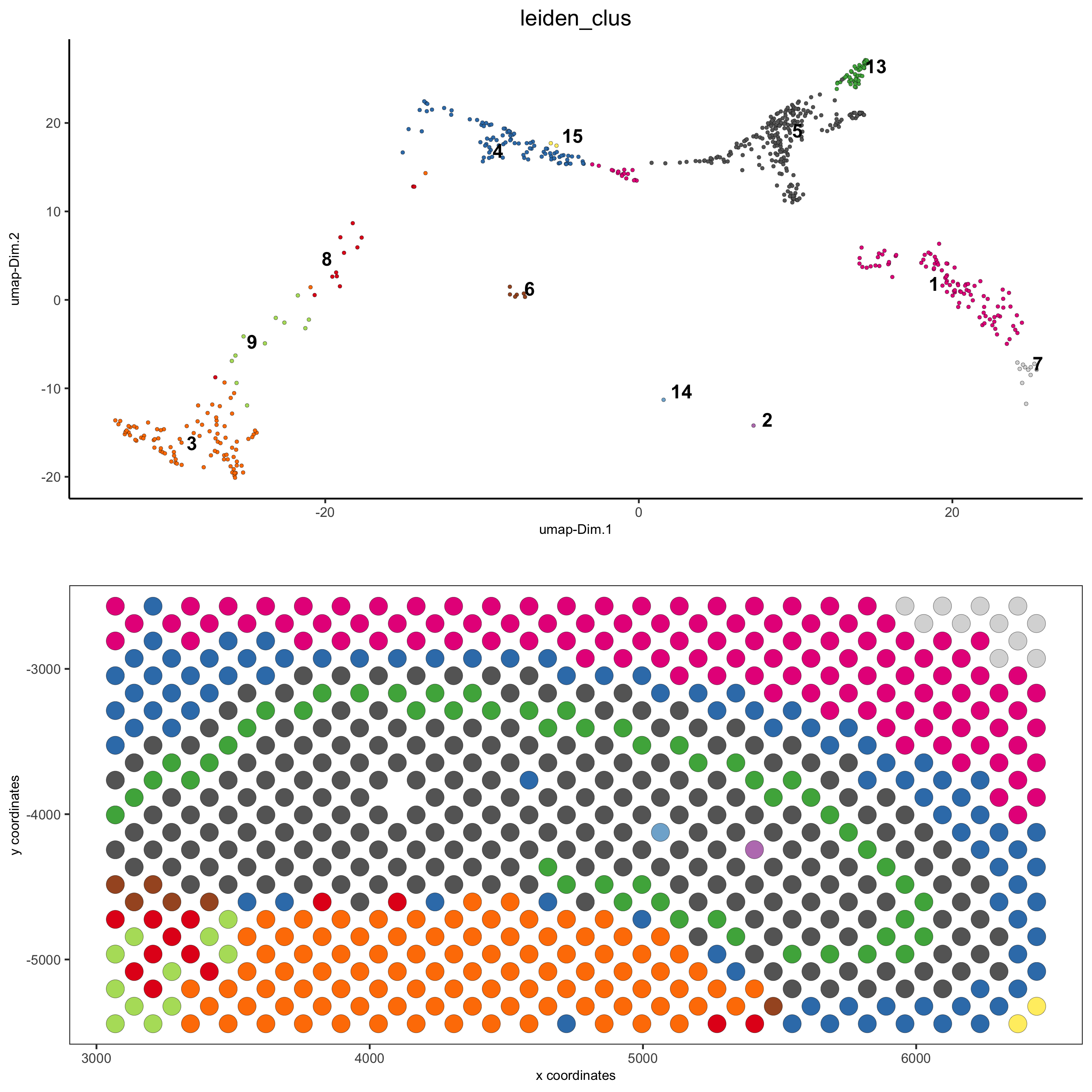
5.2 subset dataset on DG region
DG_subset = subsetGiottoLocs(visium_brain,
                             x_max = 6500, x_min = 3000, y_max = -2500, y_min = -5500,
                             return_gobject = TRUE)

spatDimPlot(gobject = DG_subset,
            cell_color = 'leiden_clus', spat_point_size = 5,
            save_param = list(save_name = '5_c_DEG_subset'))
part 6: cell type marker gene detection
gini
gini_markers_subclusters = findMarkers_one_vs_all(gobject = visium_brain,
                                                  method = 'gini',
                                                  expression_values = 'normalized',
                                                  cluster_column = 'leiden_clus',
                                                  min_genes = 20,
                                                  min_expr_gini_score = 0.5,
                                                  min_det_gini_score = 0.5)
topgenes_gini = gini_markers_subclusters[, head(.SD, 2), by = 'cluster']$genes

# violinplot
violinPlot(visium_brain, genes = unique(topgenes_gini), cluster_column = 'leiden_clus',
           strip_text = 8, strip_position = 'right',
           save_param = list(save_name = '6_a_violinplot_gini', base_width = 5, base_height = 10))
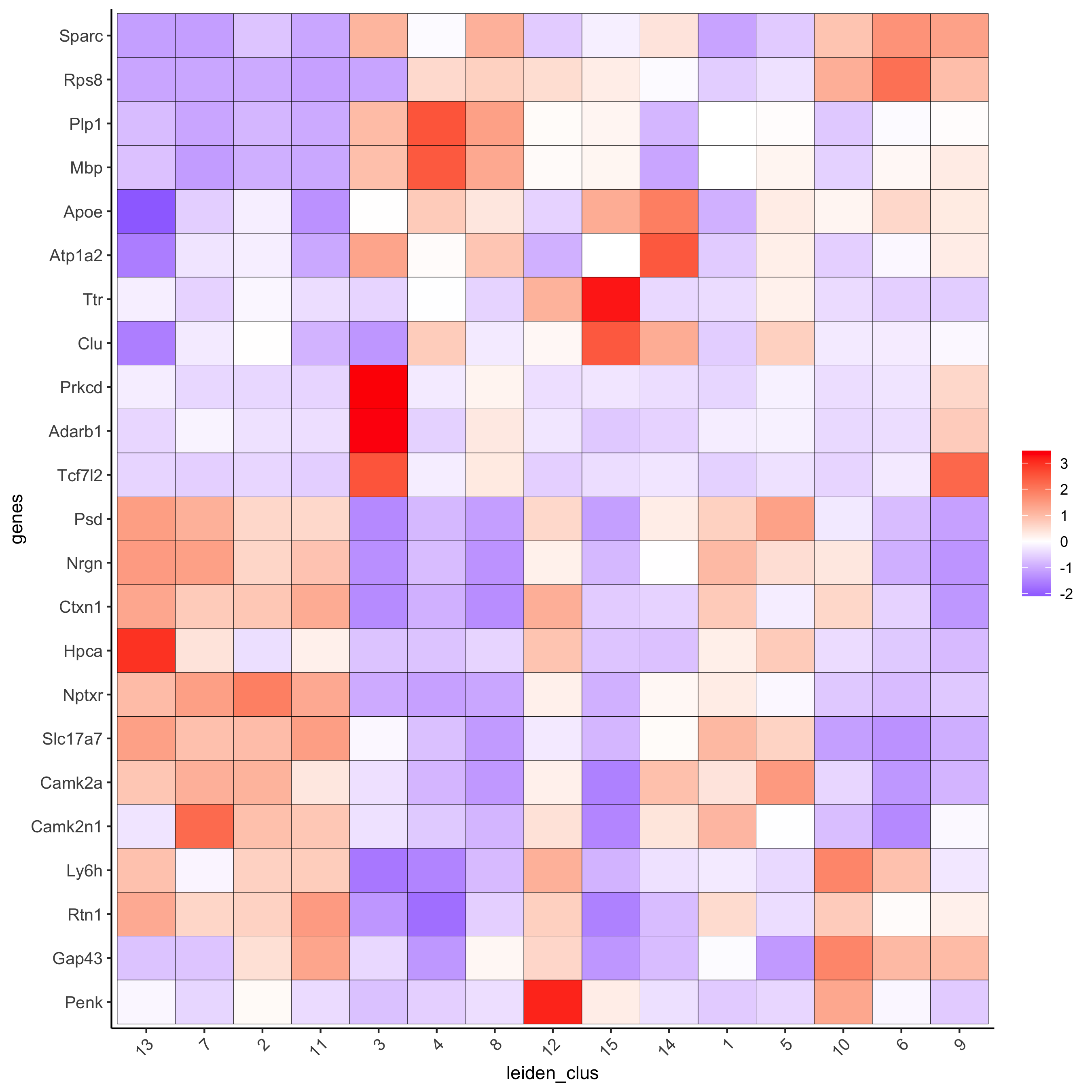
# cluster heatmap
plotMetaDataHeatmap(visium_brain, selected_genes = topgenes_gini,
                    metadata_cols = c('leiden_clus'),
                    x_text_size = 10, y_text_size = 10,
                    save_param = list(save_name = '6_b_metaheatmap_gini'))
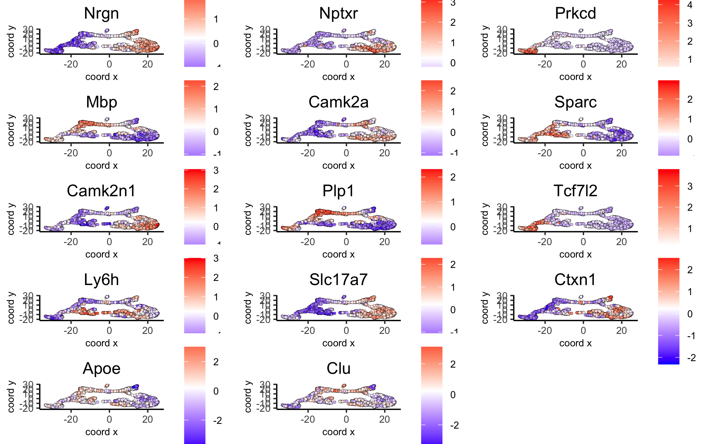
# umap plots
dimGenePlot2D(visium_brain, expression_values = 'scaled',
              genes = gini_markers_subclusters[, head(.SD, 1), by = 'cluster']$genes,
              cow_n_col = 3, point_size = 1,
              save_param = list(save_name = '6_c_gini_umap', base_width = 8, base_height = 5))
scran
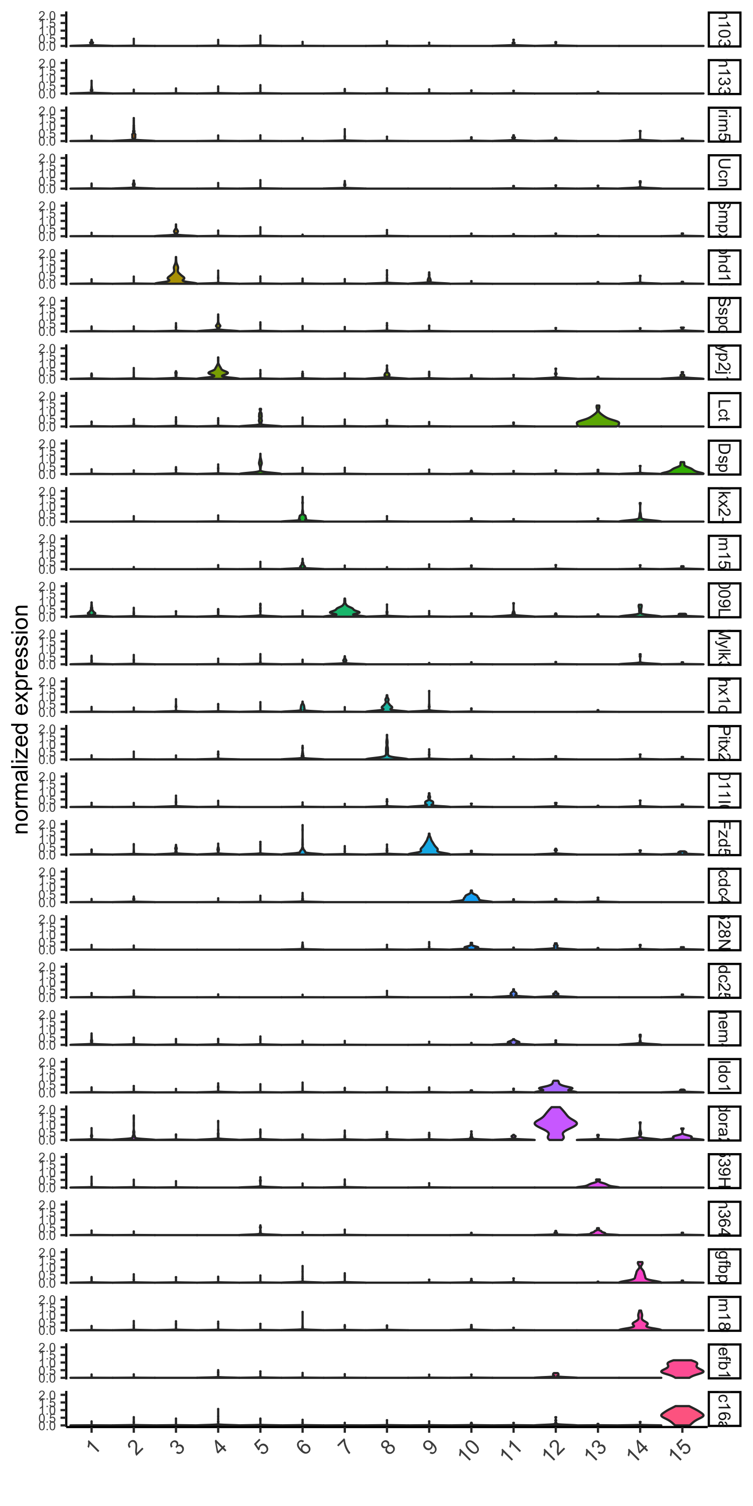
scran_markers_subclusters = findMarkers_one_vs_all(gobject = visium_brain,
                                                   method = 'scran',
                                                   expression_values = 'normalized',
                                                   cluster_column = 'leiden_clus')
topgenes_scran = scran_markers_subclusters[, head(.SD, 2), by = 'cluster']$genes

# violinplot
violinPlot(visium_brain, genes = unique(topgenes_scran), cluster_column = 'leiden_clus',
           strip_text = 10, strip_position = 'right',
           save_param = list(save_name = '6_d_violinplot_scran', base_width = 5))
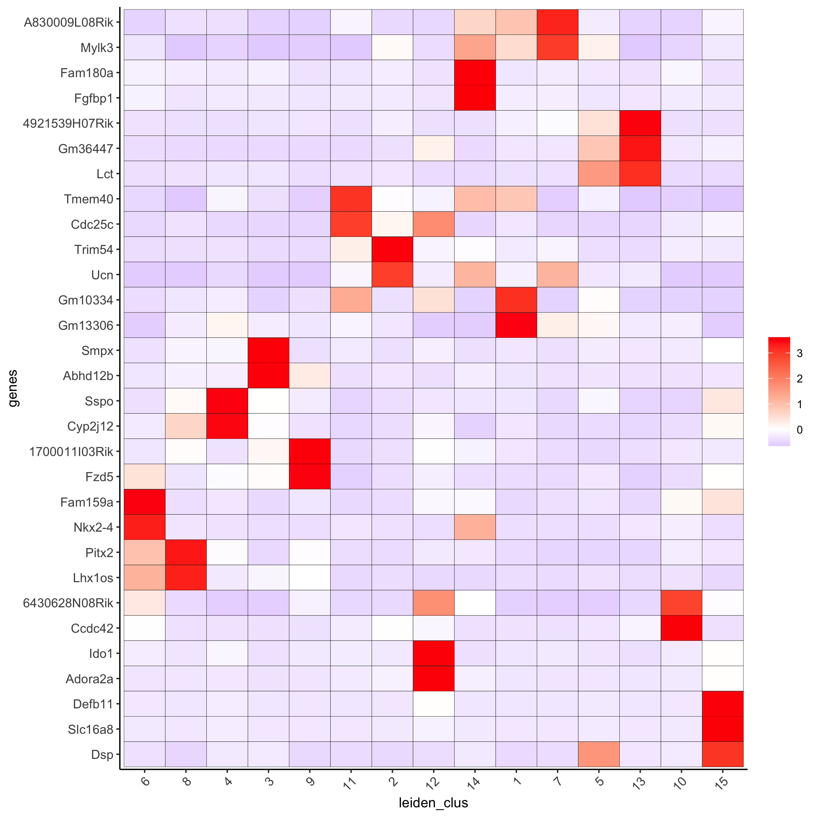
# cluster heatmap
plotMetaDataHeatmap(visium_brain, selected_genes = topgenes_scran,
                    metadata_cols = c('leiden_clus'),
                    save_param = list(save_name = '6_e_metaheatmap_scran'))
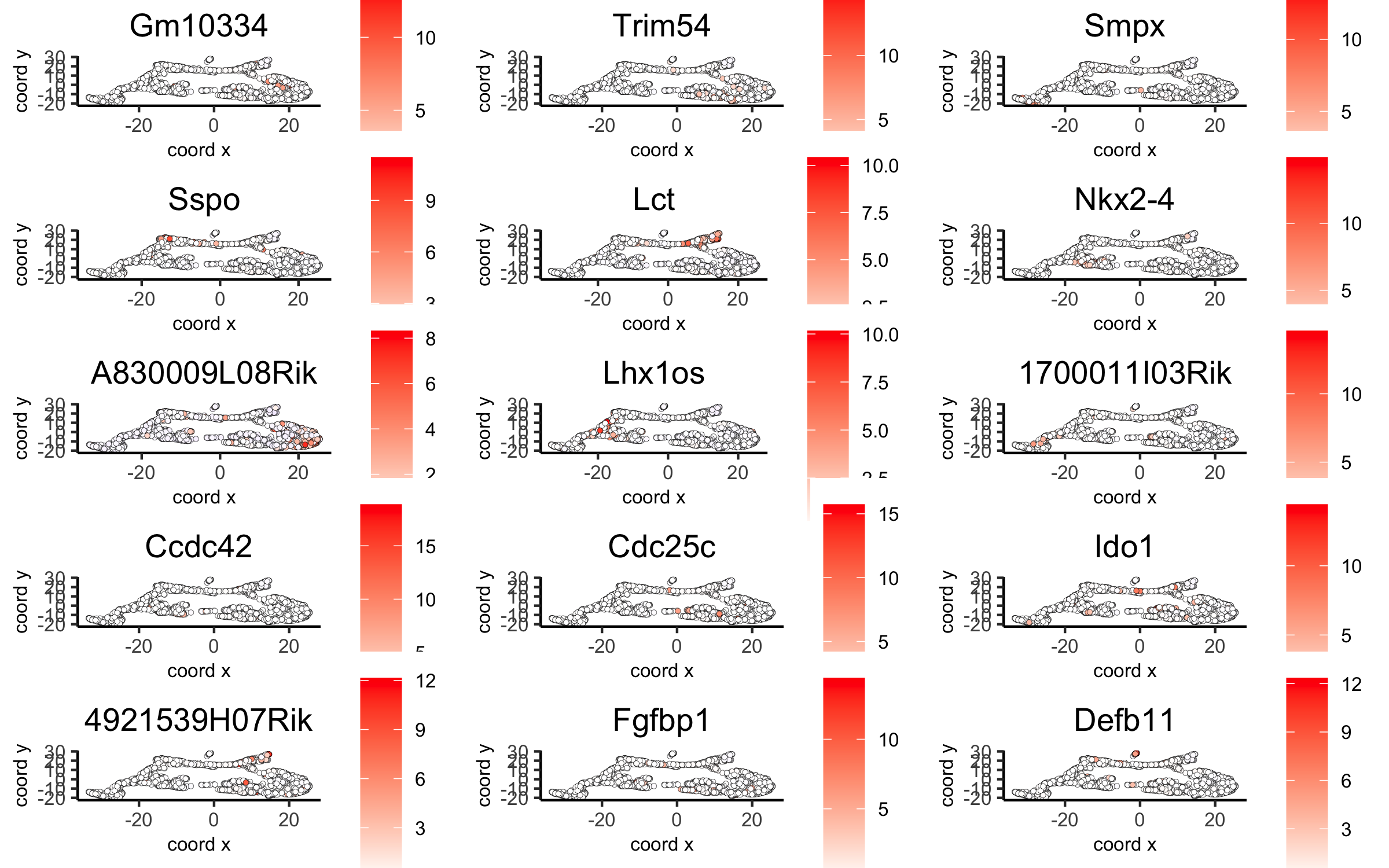
# umap plots
dimGenePlot(visium_brain, expression_values = 'scaled',
            genes = scran_markers_subclusters[, head(.SD, 1), by = 'cluster']$genes,
            cow_n_col = 3, point_size = 1,
            save_param = list(save_name = '6_f_scran_umap', base_width = 8, base_height = 5))
part 7: cell-type annotation
Visium spatial transcriptomics does not provide single-cell resolution, making cell type annotation a harder problem. Giotto provides 3 ways to calculate enrichment of specific cell-type signature gene list:
- PAGE
- rank
- hypergeometric test
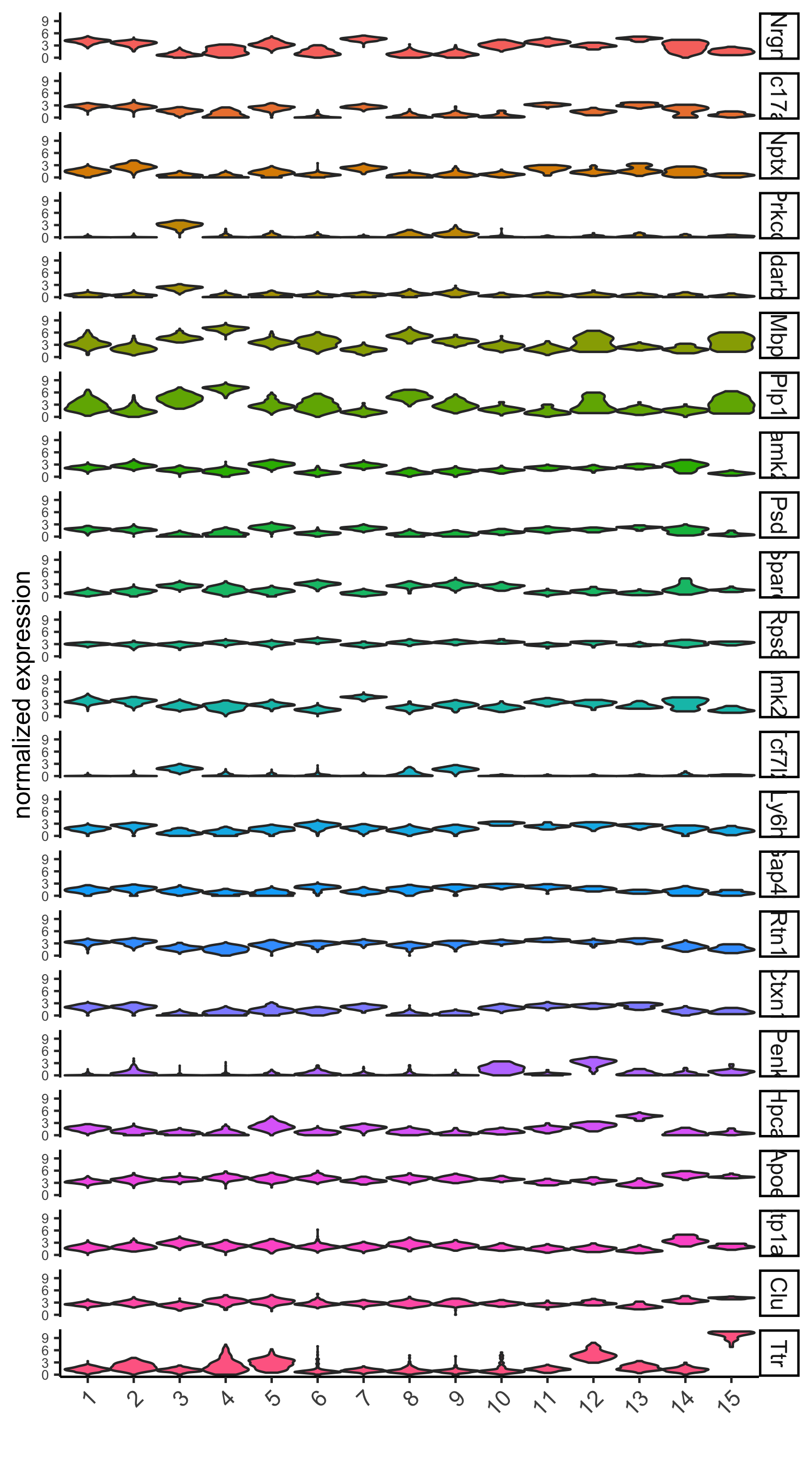
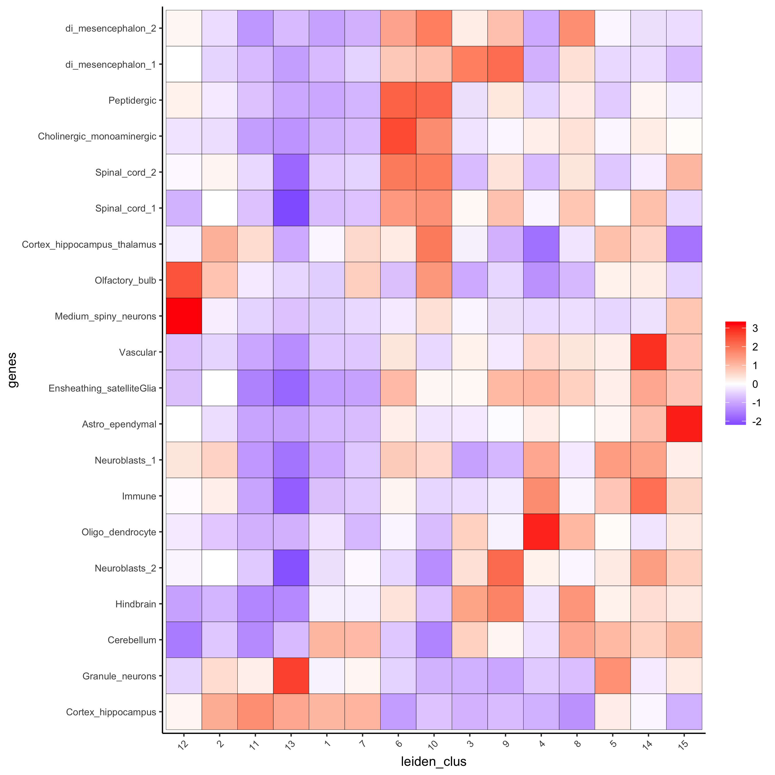
# known markers for different mouse brain cell types:
# Zeisel, A. et al. Molecular Architecture of the Mouse Nervous System. Cell 174, 999-1014.e22 (2018).
## cell type signatures ##
## combination of all marker genes identified in Zeisel et al
sign_matrix_path = system.file("extdata", "sig_matrix.txt", package = 'Giotto')
brain_sc_markers = data.table::fread(sign_matrix_path)
sig_matrix = as.matrix(brain_sc_markers[,-1]); rownames(sig_matrix) = brain_sc_markers$Event

## enrichment tests
visium_brain = createSpatialEnrich(visium_brain, sign_matrix = sig_matrix, enrich_method = 'PAGE')

## heatmap of enrichment versus annotation (e.g. clustering result)
cell_types = colnames(sig_matrix)
plotMetaDataCellsHeatmap(gobject = visium_brain,
                         metadata_cols = 'leiden_clus',
                         value_cols = cell_types,spat_enr_names = 'PAGE',
                         x_text_size = 8, y_text_size = 8,
                         save_param = list(save_name="7_a_metaheatmap"))
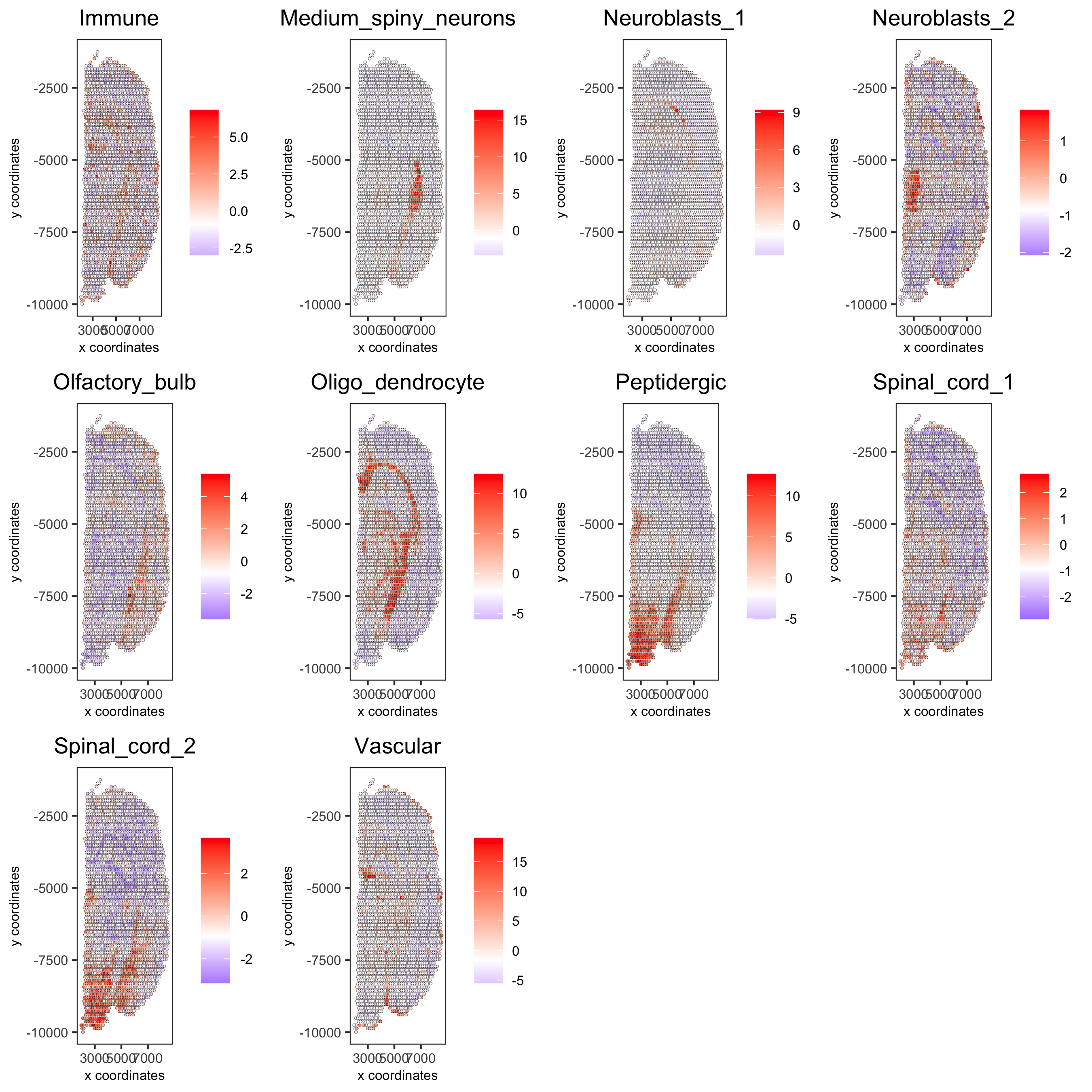
cell_types_subset = colnames(sig_matrix)[1:10]
spatCellPlot(gobject = visium_brain,
             spat_enr_names = 'PAGE',cell_annotation_values = cell_types_subset,
             cow_n_col = 4,coord_fix_ratio = NULL, point_size = 0.75,
             save_param = list(save_name="7_b_spatcellplot_1"))
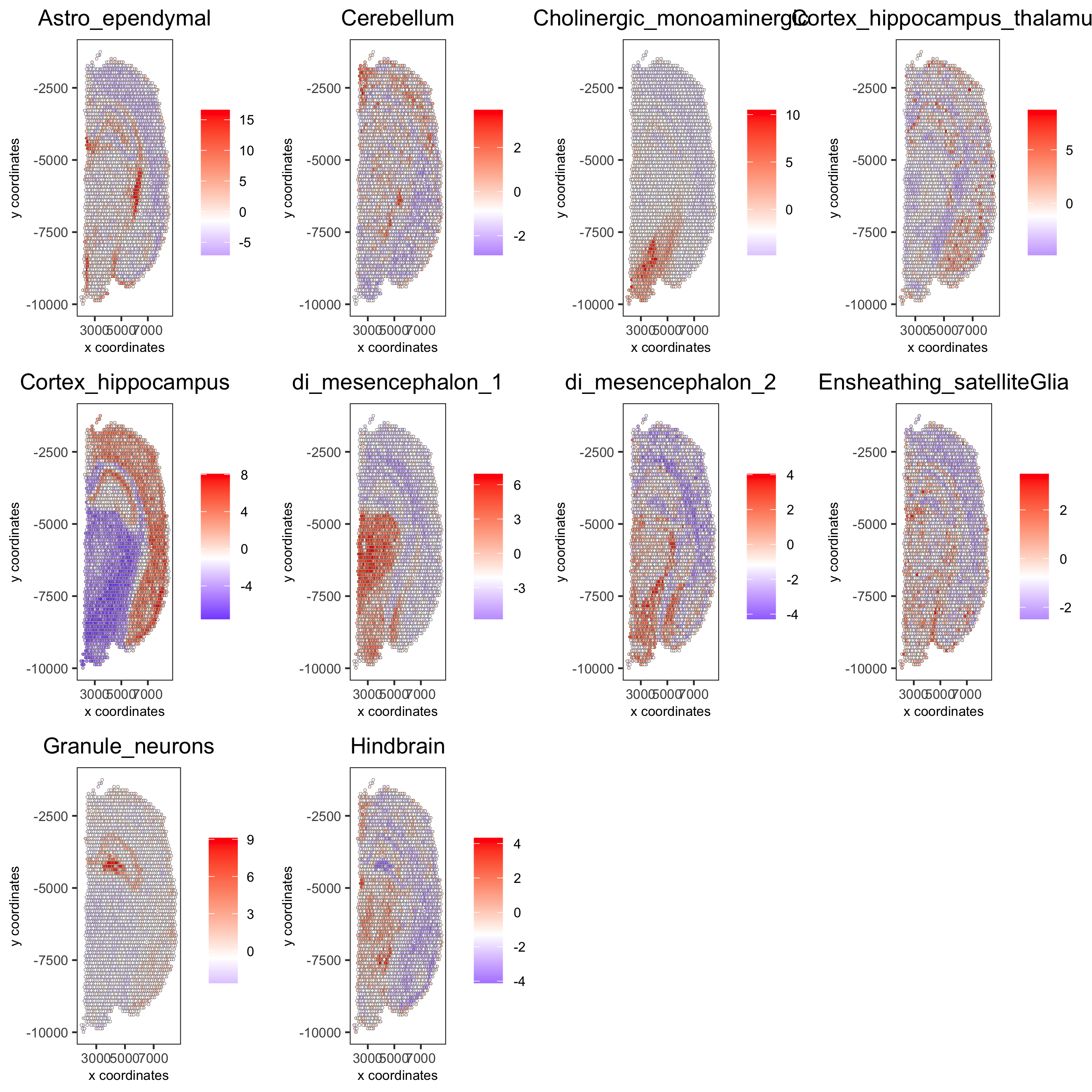
cell_types_subset = colnames(sig_matrix)[11:20]
spatCellPlot(gobject = visium_brain, spat_enr_names = 'PAGE',
             cell_annotation_values = cell_types_subset, cow_n_col = 4,
             coord_fix_ratio = NULL, point_size = 0.75,
             save_param = list(save_name="7_c_spatcellplot_2"))
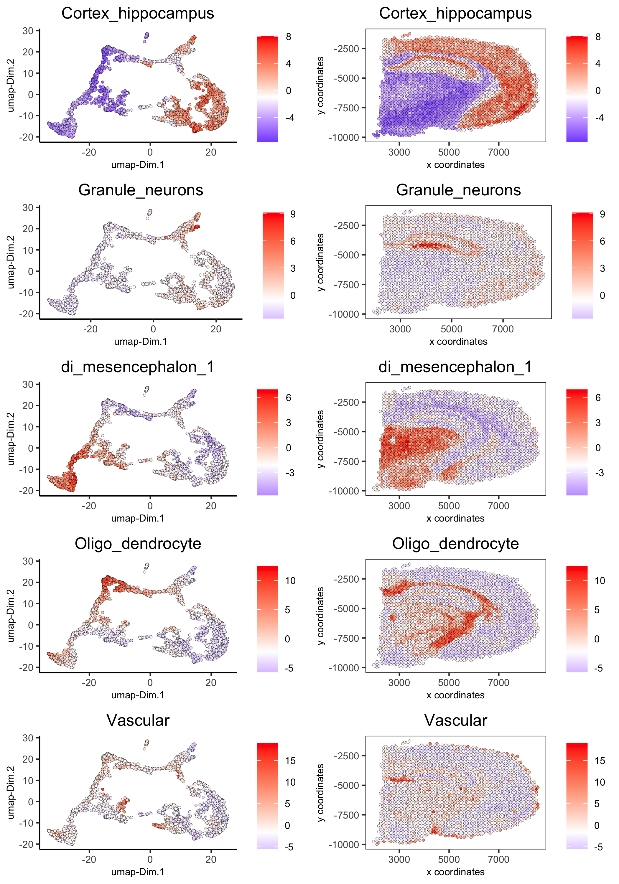
spatDimCellPlot(gobject = visium_brain,
                spat_enr_names = 'PAGE',
                cell_annotation_values = c('Cortex_hippocampus', 'Granule_neurons', 'di_mesencephalon_1', 'Oligo_dendrocyte','Vascular'),
                cow_n_col = 1, spat_point_size = 1,
                plot_alignment = 'horizontal',
                save_param = list(save_name="7_d_spatDimCellPlot", base_width=7, base_height=10))
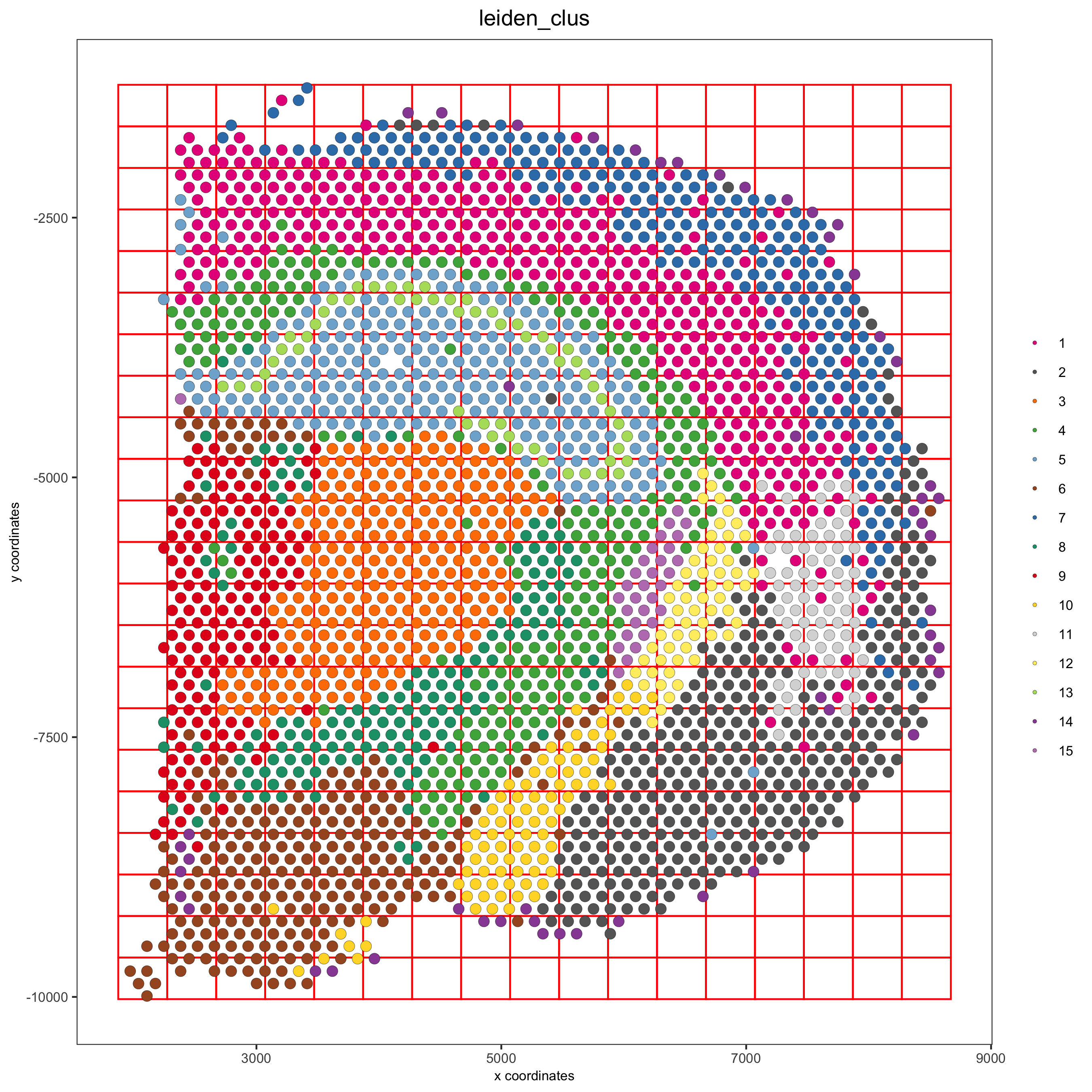
part 8: spatial grid
visium_brain <- createSpatialGrid(gobject = visium_brain,
                                   sdimx_stepsize = 400,
                                   sdimy_stepsize = 400,
                                   minimum_padding = 0)
spatPlot(visium_brain, cell_color = 'leiden_clus', show_grid = T,
         grid_color = 'red', spatial_grid_name = 'spatial_grid',
         save_param = list(save_name = '8_grid'))
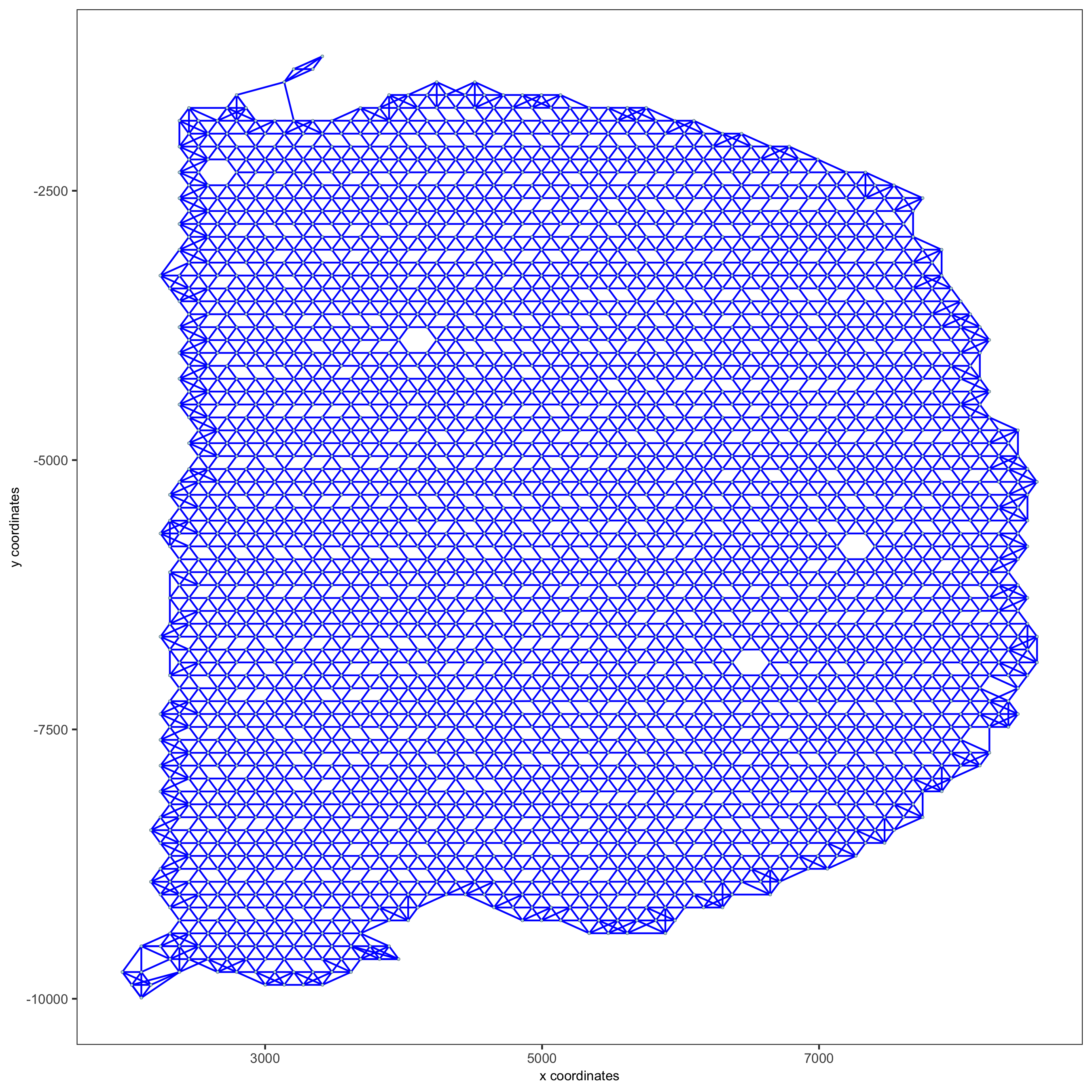
part 9: spatial network
visium_brain <- createSpatialNetwork(gobject = visium_brain,
                                     method = 'kNN', k = 5,
                                     maximum_distance_knn = 400,
                                     name = 'spatial_network')

showNetworks(visium_brain)

spatPlot(gobject = visium_brain, show_network = T,
         network_color = 'blue', spatial_network_name = 'spatial_network',
         save_param = list(save_name = '9_a_knn_network'))
part 10: spatial genes
Spatial genes
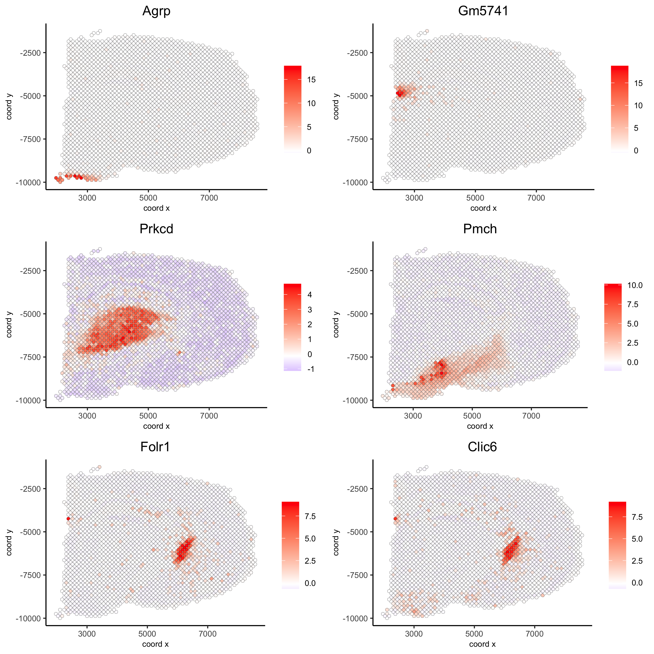
## kmeans binarization
kmtest = binSpect(visium_brain, calc_hub = T, hub_min_int = 5,
                  spatial_network_name = 'spatial_network')
spatGenePlot(visium_brain, expression_values = 'scaled',
             genes = kmtest$genes[1:6], cow_n_col = 2, point_size = 1.5,
             save_param = list(save_name = '10_a_spatial_genes_km'))
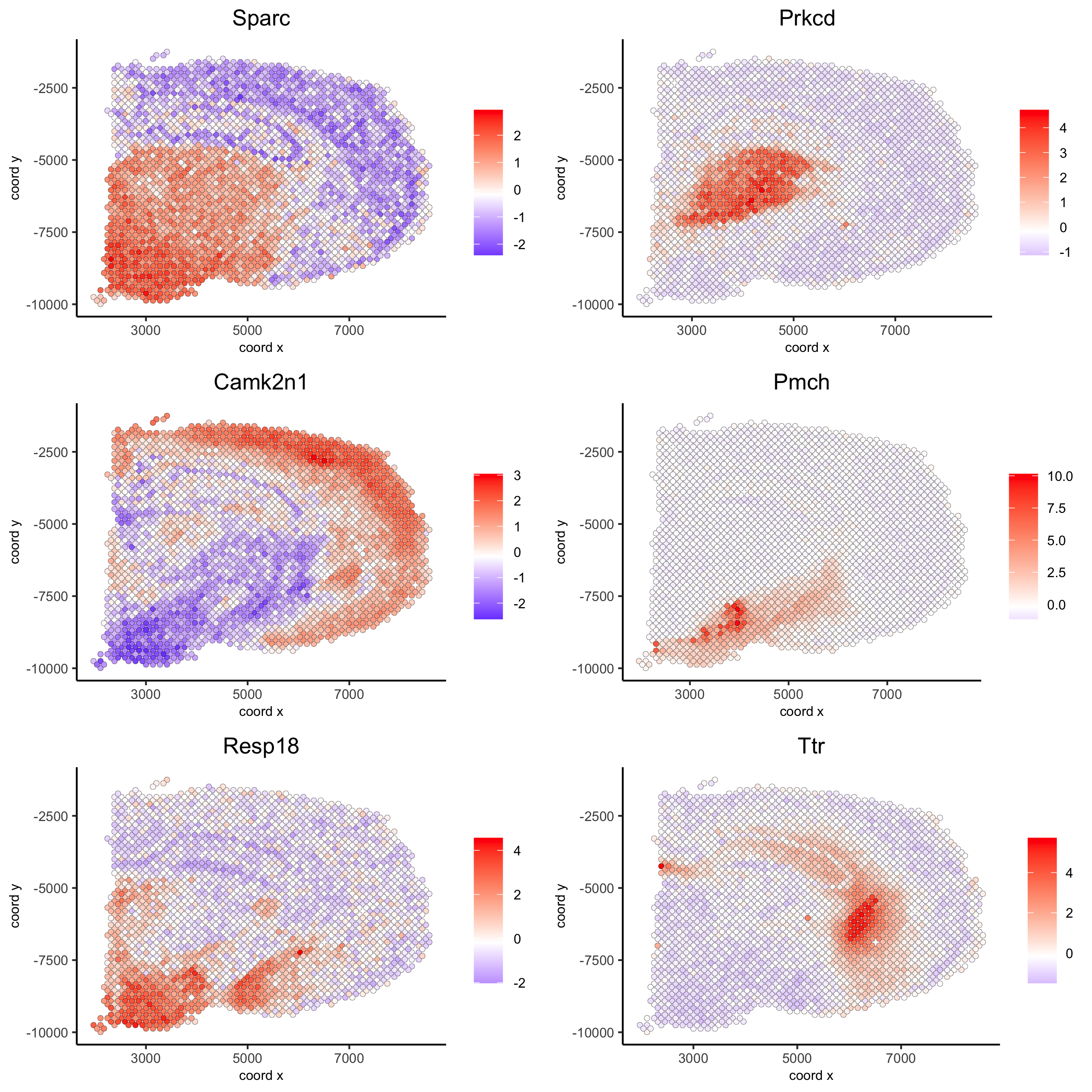
## rank binarization
ranktest = binSpect(visium_brain, bin_method = 'rank',
                    calc_hub = T, hub_min_int = 5,
                    spatial_network_name = 'spatial_network')
spatGenePlot(visium_brain, expression_values = 'scaled',
             genes = ranktest$genes[1:6], cow_n_col = 2, point_size = 1.5,
             save_param = list(save_name = '10_b_spatial_genes_rank'))
![]()
spatial_genes = silhouetteRankTest(gobject = visium_brain,
                               expression_values = 'scaled',
                               rbp_ps = c(0.95, 0.99), examine_tops = c(0.1, 0.3),
                               parallel_path = "/usr/local/bin")
spatGenePlot(visium_brain, expression_values = 'scaled',
             genes = spatial_genes$gene[1:6], cow_n_col = 2, point_size = 1,
             save_param = list(save_name = '10_c_silhouette'))
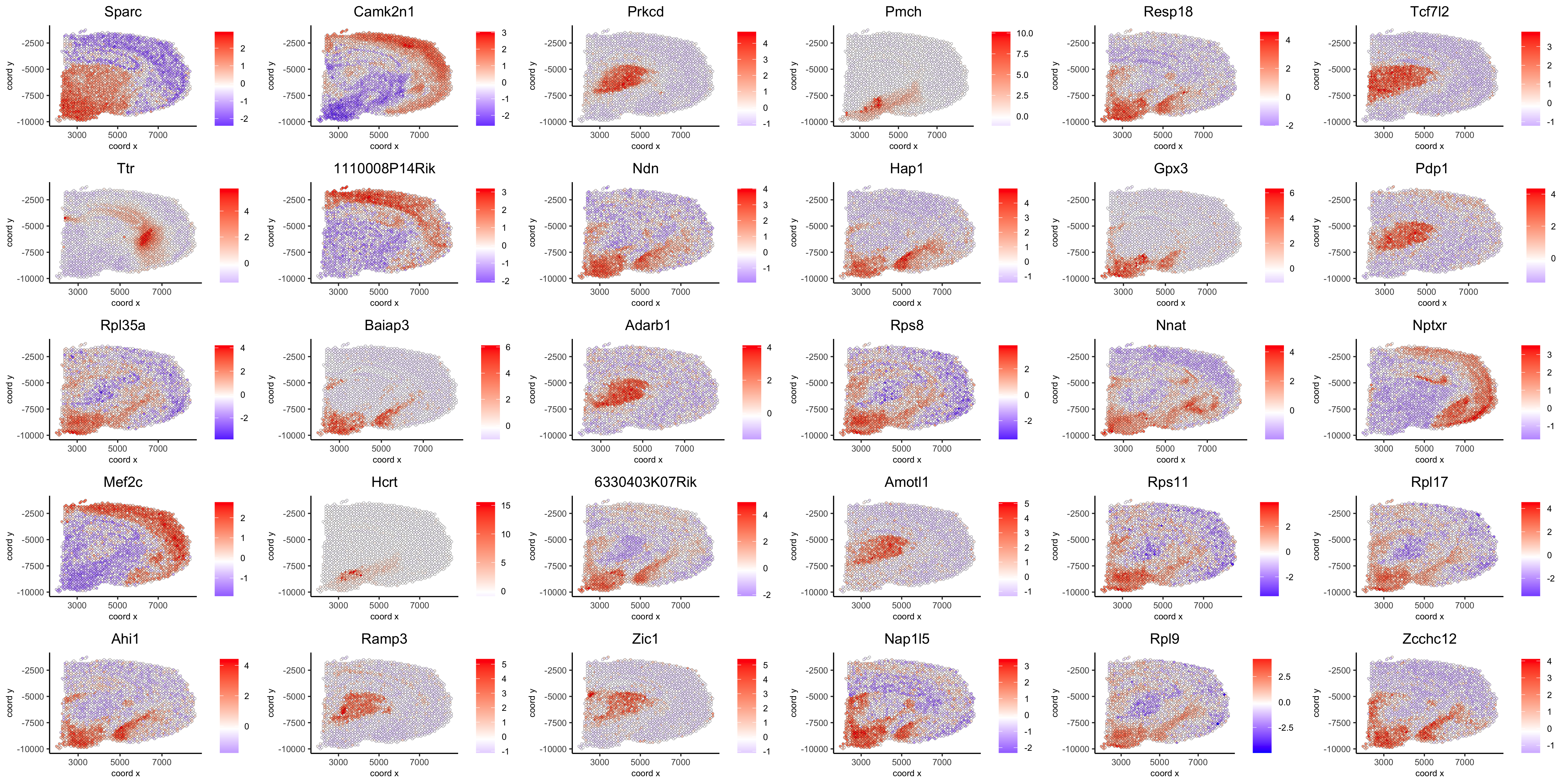
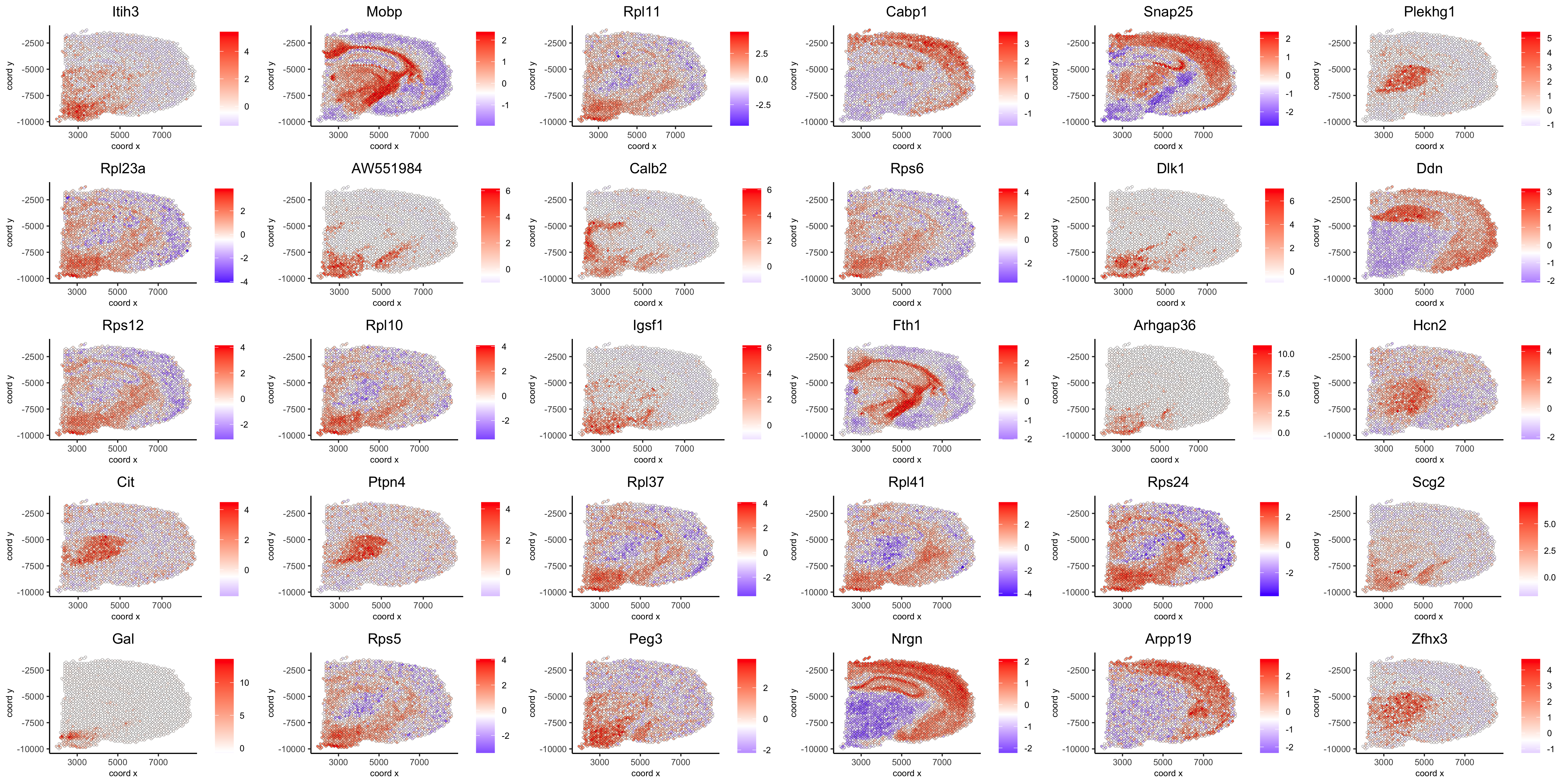
show top 90 genes identified by silhouetteRank:
spatGenePlot(visium_brain, expression_values = 'scaled',
             genes = spatial_genes$gene[1:30],
             cow_n_col = 6, point_size = 1,
             save_param = list(save_name="10_d_silhouette_1", base_width=20, base_height=10))
spatGenePlot(visium_brain, expression_values = 'scaled',
             genes = spatial_genes$gene[31:60],
             cow_n_col = 6, point_size = 1,
             save_param = list(save_name="10_d_silhouette_2", base_width=20, base_height=10))
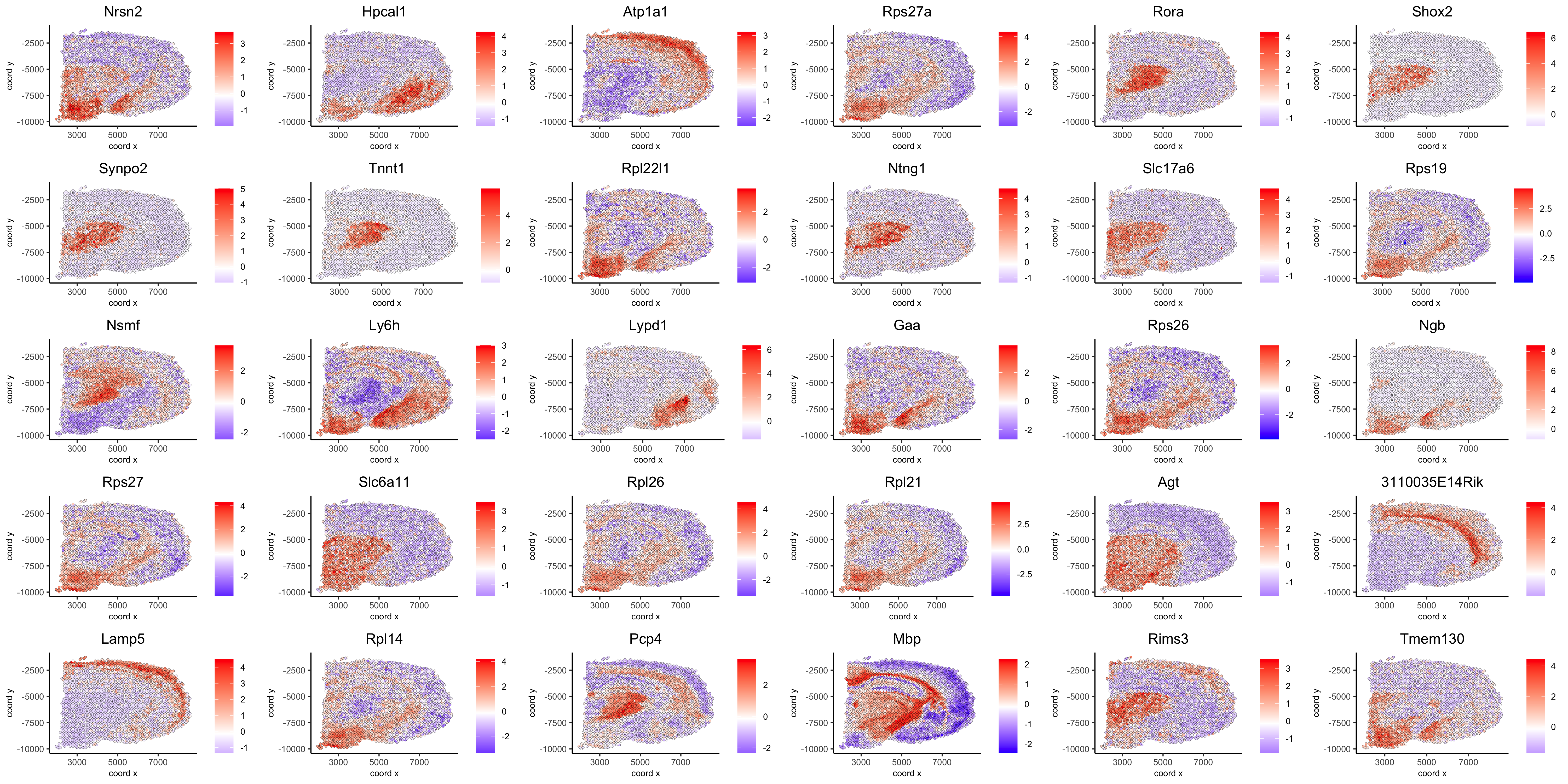
spatGenePlot(visium_brain, expression_values = 'scaled',
             genes = spatial_genes$gene[61:90],
             cow_n_col = 6, point_size = 1,
             save_param = list(save_name="10_d_silhouette_3", base_width=20, base_height=10))
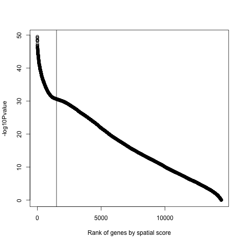
png(filename = paste0(results_folder,'/', '10_e_plot.png'))
plot(x=seq(1, 14414),
     y=-log10(spatial_genes$pval),
     xlab="Rank of genes by spatial score",
     ylab="-log10Pvalue")
abline(v=c(1500))
dev.off()
Spatial patterns
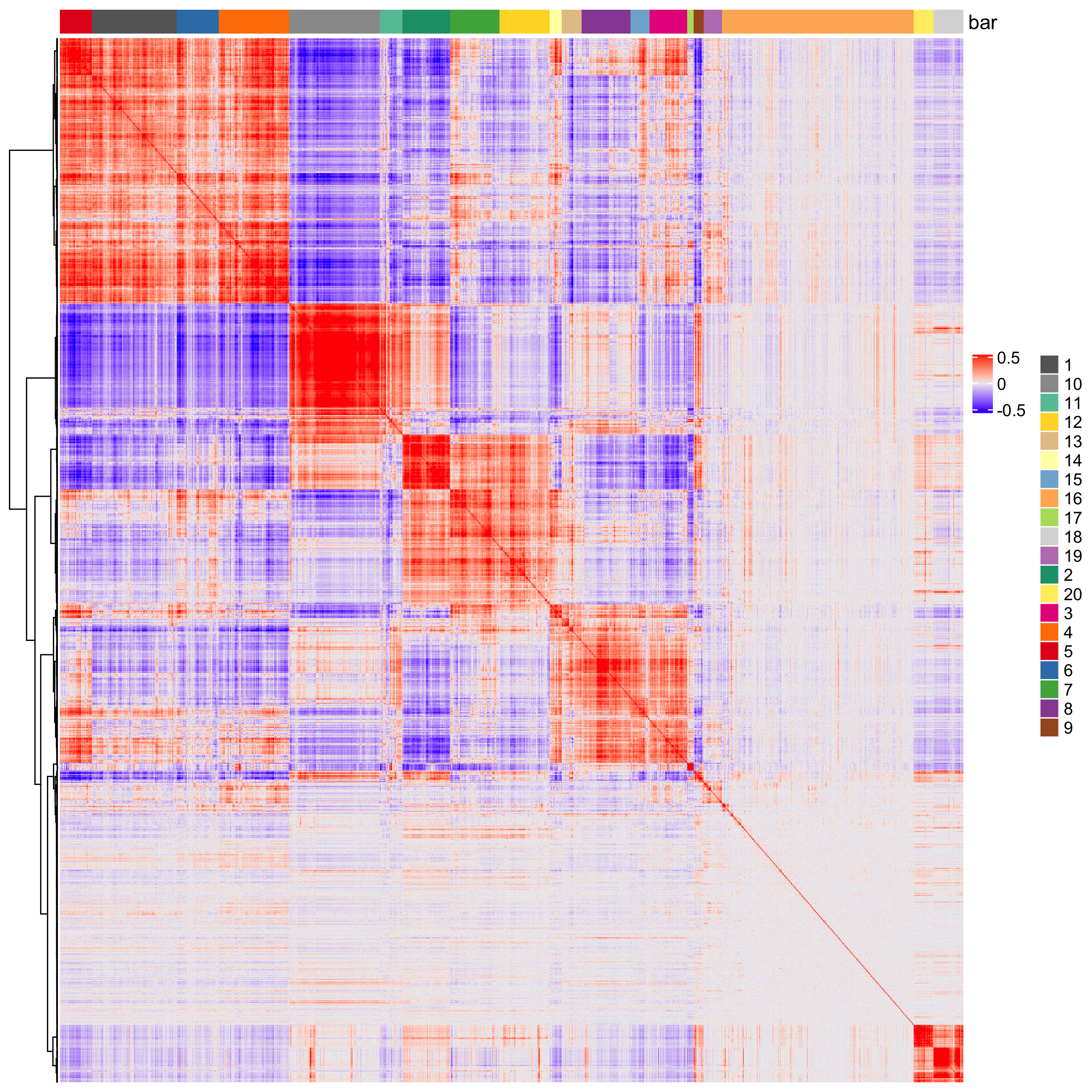
# cluster the top 1500 spatial genes into 20 clusters
ext_spatial_genes = spatial_genes[1:1500,]$gene

# here we use existing detectSpatialCorGenes function to calculate pairwise distances between genes (but set network_smoothing=0 to use default clustering)
spat_cor_netw_DT = detectSpatialCorGenes(visium_brain,
                                         method = 'network',
                                         spatial_network_name = 'spatial_network',
                                         subset_genes = ext_spatial_genes, network_smoothing=0)

# cluster spatial genes
spat_cor_netw_DT = clusterSpatialCorGenes(spat_cor_netw_DT, name = 'spat_netw_clus', k = 20)

# visualize clusters
heatmSpatialCorGenes(visium_brain,
                     spatCorObject = spat_cor_netw_DT,
                     use_clus_name = 'spat_netw_clus',
                     heatmap_legend_param = list(title = NULL),
                     save_param = list(save_name="10_e_heatmap"))
# sample the spatial genes at a per cluster basis
# but different from regular sampling, sampling is based on cluster size
# controlled by sample_rate (between 1 to 10. 1 means equal number per cluster, 10 means number of samples is directly proportional to cluster size)
# target number of spatial genes = 500

# extract cluster information
clusters = spat_cor_netw_DT$cor_clusters
clust = clusters$spat_netw_clus

sample_rate=2
target=500
tot=0
num_cluster=20
gene_list = list()
for(i in seq(1, num_cluster)){
    gene_list[[i]] = colnames(t(clust[which(clust==i)]))
}
for(i in seq(1, num_cluster)){
    num_g=length(gene_list[[i]])
    tot = tot+num_g/(num_g^(1/sample_rate))
}
factor=target/tot
num_sample=c()
for(i in seq(1, num_cluster)){
    num_g=length(gene_list[[i]])
    num_sample[i] = round(num_g/(num_g^(1/sample_rate)) * factor)
}
set.seed(10)
samples=list()
union_genes = c()
for(i in seq(1, num_cluster)){
    if(length(gene_list[[i]])<num_sample[i]){
        samples[[i]] = gene_list[[i]]
    }else{
        samples[[i]] = sample(gene_list[[i]], num_sample[i])
    }
    union_genes = union(union_genes, samples[[i]])
}
union_genes = unique(union_genes)
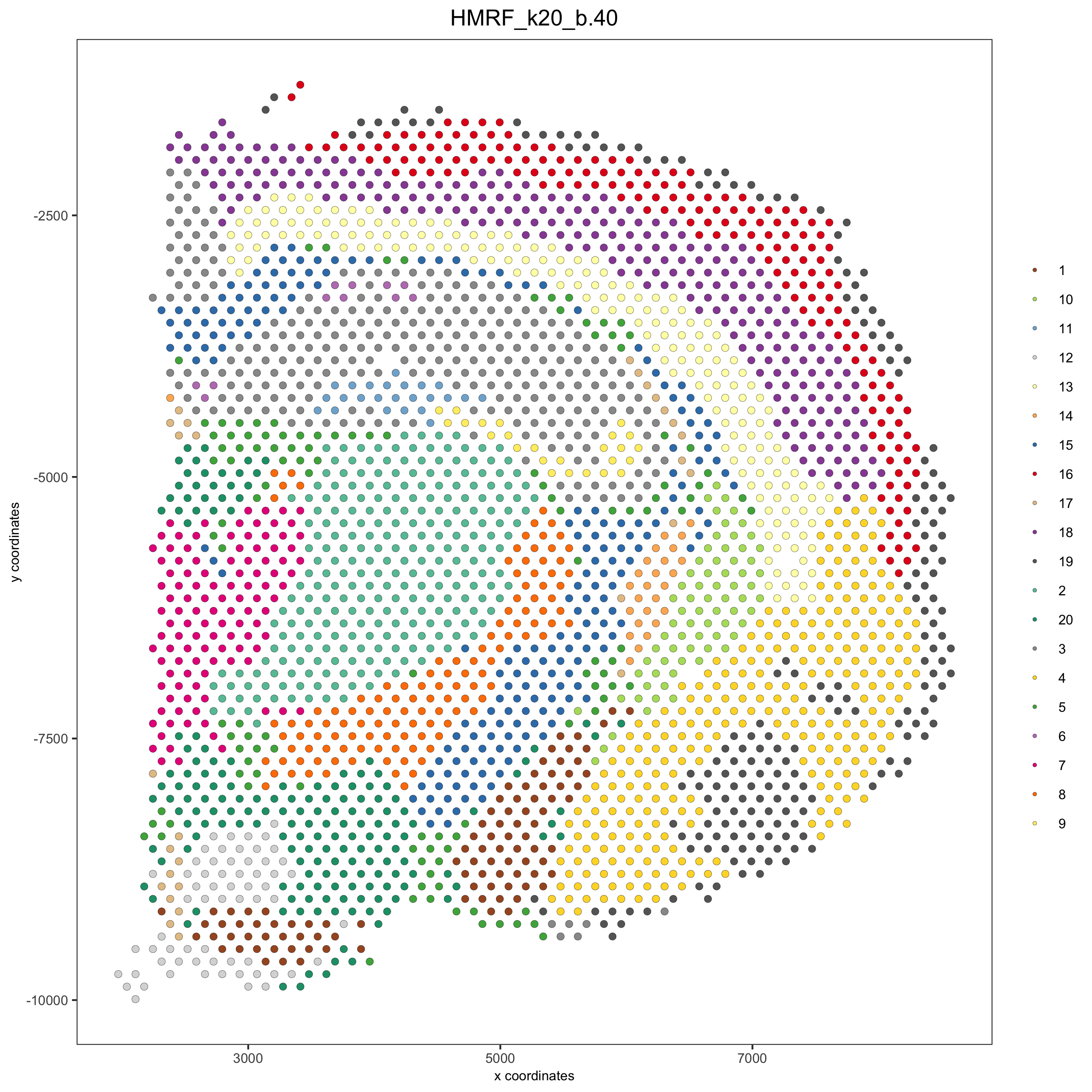
# do HMRF with different betas on 500 spatial genes
my_spatial_genes <- union_genes

hmrf_folder = paste0(results_folder,'/','11_HMRF/')
if(!file.exists(hmrf_folder)) dir.create(hmrf_folder, recursive = T)

HMRF_spatial_genes = doHMRF(gobject = visium_brain,
                            expression_values = 'scaled',
                            spatial_genes = my_spatial_genes, k = 20,
                            spatial_network_name="spatial_network",
                            betas = c(0, 10, 5),
                            output_folder = paste0(hmrf_folder, '/', 'Spatial_genes/SG_topgenes_k20_scaled'))

visium_brain = addHMRF(gobject = visium_brain, HMRFoutput = HMRF_spatial_genes,
                       k = 20, betas_to_add = c(0, 10, 20, 30, 40),
                       hmrf_name = 'HMRF')

spatPlot(gobject = visium_brain, cell_color = 'HMRF_k20_b.40',
         point_size = 2, save_param=c(save_name="10_d_spatPlot2D_HMRF"))
Export and create Giotto Viewer
# check which annotations are available
combineMetadata(visium_brain, spat_enr_names = 'PAGE')

# select annotations, reductions and expression values to view in Giotto Viewer
viewer_folder = paste0(results_folder, '/', 'mouse_Visium_brain_viewer')

exportGiottoViewer(gobject = visium_brain,
                   output_directory = viewer_folder,
                   spat_enr_names = 'PAGE',
                   factor_annotations = c('in_tissue',
                                          'leiden_clus',
                                          'HMRF_k20_b.40'),
                   numeric_annotations = c('nr_genes',
                                           'clus_25'),
                   dim_reductions = c('tsne', 'umap'),
                   dim_reduction_names = c('tsne', 'umap'),
                   expression_values = 'scaled',
                   expression_rounding = 2,
                   overwrite_dir = T)