STARmap mouse cortex
Source:vignettes/mouse_starmap_cortex_200917.Rmd
mouse_starmap_cortex_200917.Rmd#> Warning: This tutorial was written with Giotto version 0.3.6.9042, your version
#> is 1.1.2.This is a more recent version and results should be reproducible
library(Giotto)

# 1. set working directory
results_folder = '/path/to/directory/'

# 2. set giotto python path
# set python path to your preferred python version path
# set python path to NULL if you want to automatically install (only the 1st time) and use the giotto miniconda environment
python_path = NULL
if(is.null(python_path)) {
  installGiottoEnvironment()
}
Dataset explanation
Wang et al. created a 3D spatial expression dataset consisting of 28 genes from 32,845 single cells in a visual cortex volume using the STARmap technology.
The STARmap data to run this tutorial can be found here. Alternatively you can use the getSpatialDataset to automatically download this dataset like we do in this example.
Dataset download
# download data to working directory
# if wget is installed, set method = 'wget'
# if you run into authentication issues with wget, then add " extra = '--no-check-certificate' "
getSpatialDataset(dataset = 'starmap_3D_cortex', directory = results_folder, method = 'wget')
Part 1: Giotto global instructions and preparations
## instructions allow us to automatically save all plots into a chosen results folder
instrs = createGiottoInstructions(show_plot = FALSE,
                                  save_plot = TRUE,
                                  save_dir = results_folder,
                                  python_path = python_path)

expr_path = paste0(results_folder, "STARmap_3D_data_expression.txt")
loc_path = paste0(results_folder, "STARmap_3D_data_cell_locations.txt")
part 2: Create Giotto object & process data
## create
STAR_test <- createGiottoObject(raw_exprs = expr_path,
                                spatial_locs = loc_path,
                                instructions = instrs)

## filter raw data
# pre-test filter parameters
filterDistributions(STAR_test, detection = 'genes',
                    save_param = list(save_name = '2_a_distribution_genes'))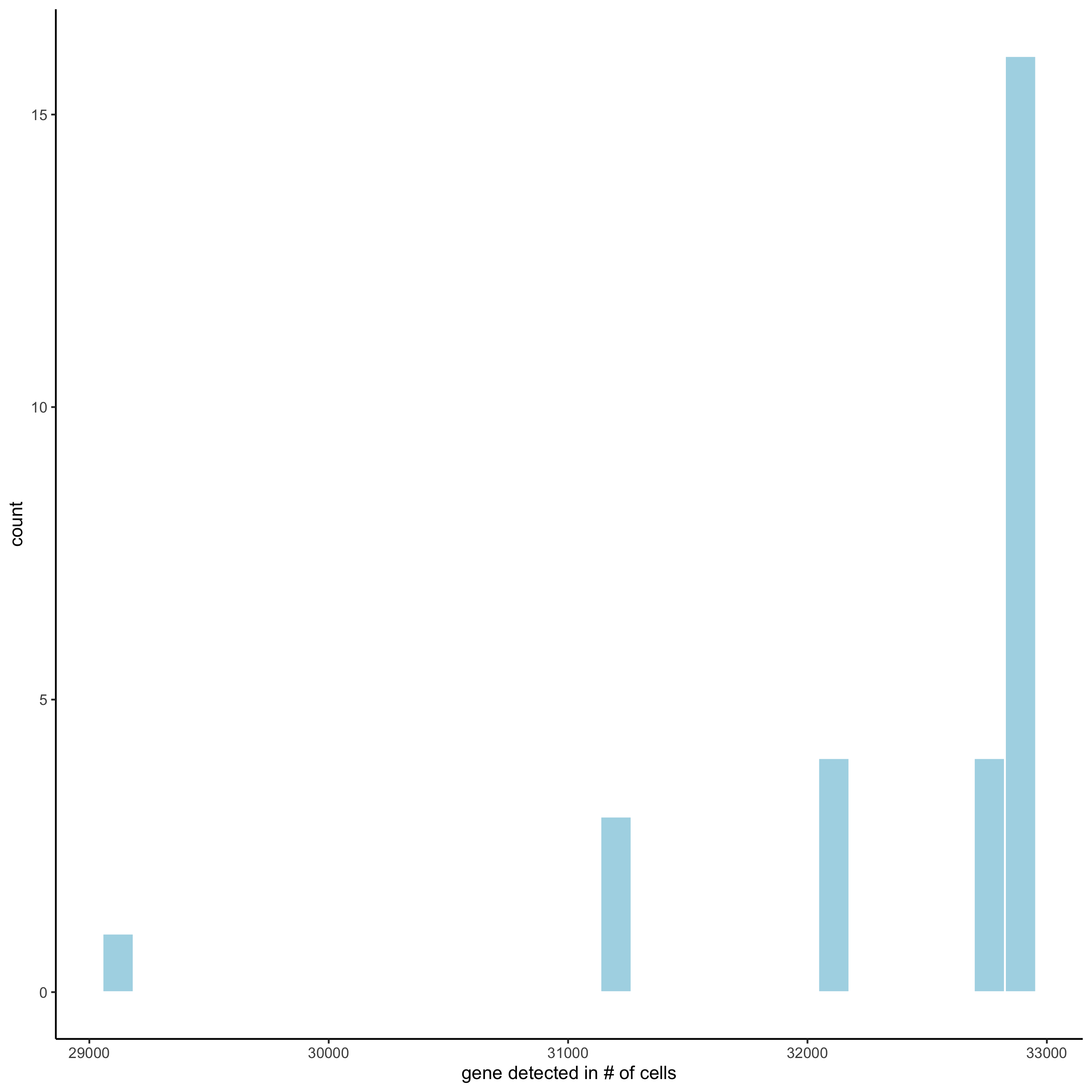
filterDistributions(STAR_test, detection = 'cells',
                    save_param = list(save_name = '2_b_distribution_cells'))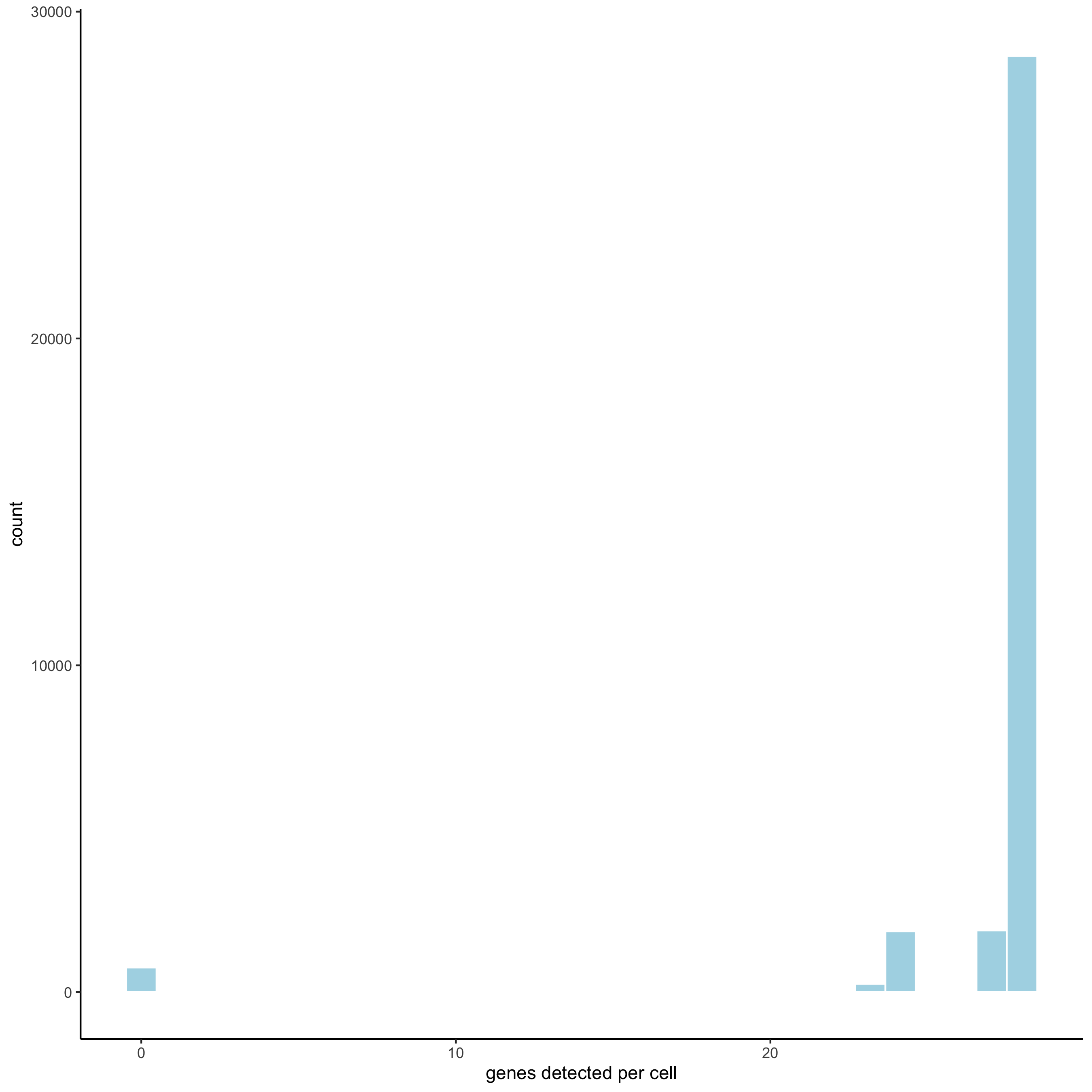
filterCombinations(STAR_test, expression_thresholds = c(1, 1,2),
                   gene_det_in_min_cells = c(20000, 20000, 30000),
                   min_det_genes_per_cell = c(10, 20, 25),
                   save_param = list(save_name = '2_c_distribution_filters'))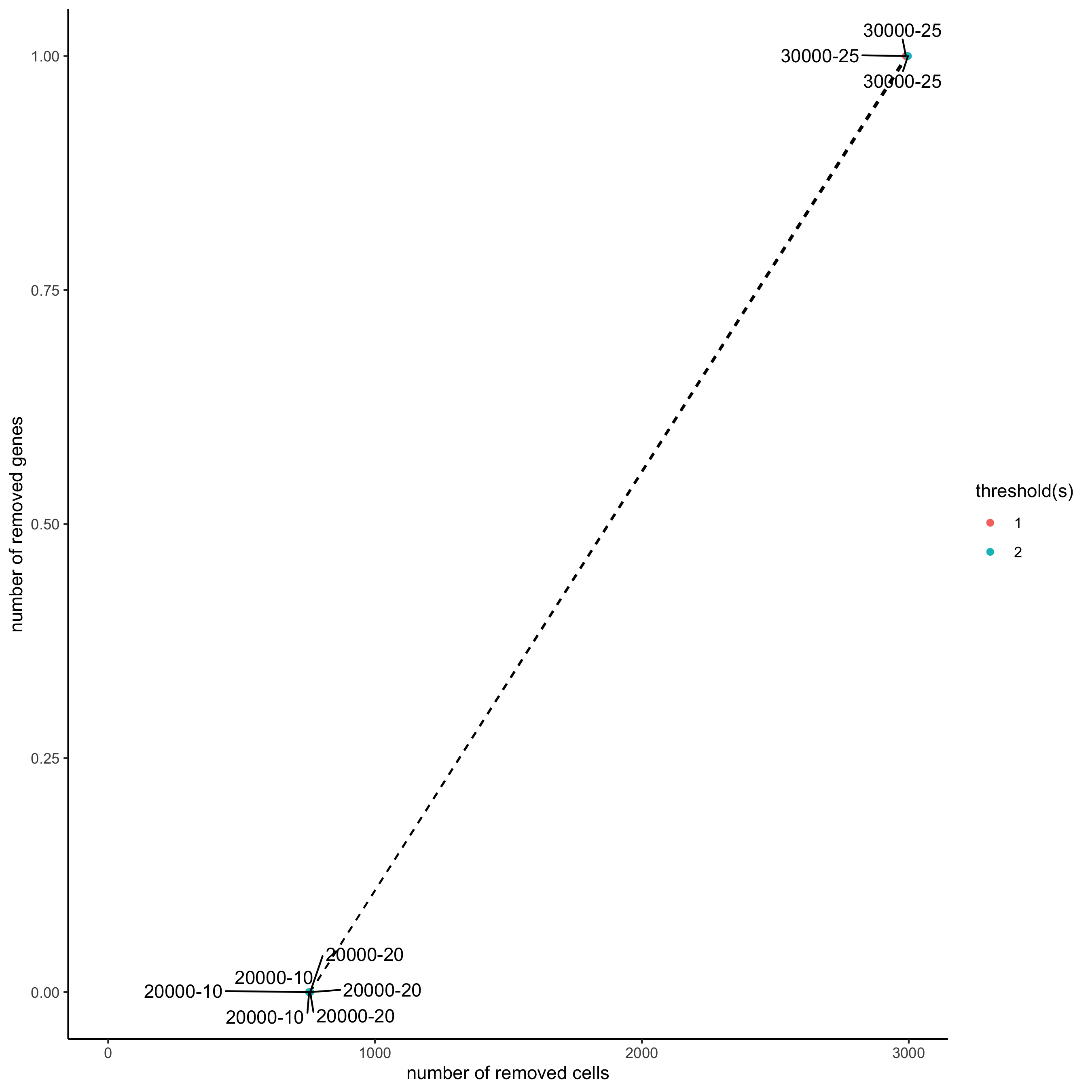
# filter
STAR_test <- filterGiotto(gobject = STAR_test,
                          gene_det_in_min_cells = 20000,
                          min_det_genes_per_cell = 20)
## normalize
STAR_test <- normalizeGiotto(gobject = STAR_test, scalefactor = 10000, verbose = T)
STAR_test <- addStatistics(gobject = STAR_test)
STAR_test <- adjustGiottoMatrix(gobject = STAR_test, expression_values = c('normalized'),
                                batch_columns = NULL, covariate_columns = c('nr_genes', 'total_expr'),
                                return_gobject = TRUE,
                                update_slot = c('custom'))
## visualize
# 3D
spatPlot3D(gobject = STAR_test, point_size = 2,
           save_param = list(save_name = '2_d_spatplot_3D'))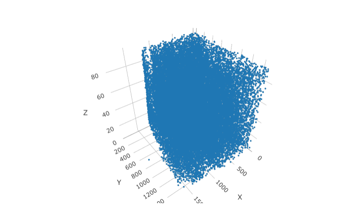
part 3: dimension reduction
STAR_test <- calculateHVG(gobject = STAR_test, method = 'cov_groups',
                          zscore_threshold = 0.5, nr_expression_groups = 3,
                          save_param = list(save_name = '3_a_HVGplot', base_height = 5, base_width = 5))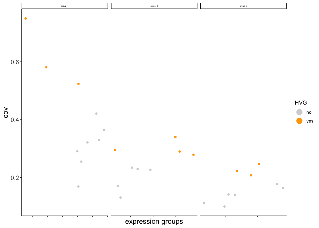
# too few highly variable genes
# genes_to_use = NULL is the default and will use all genes available
STAR_test <- runPCA(gobject = STAR_test, genes_to_use = NULL, scale_unit = F,method = 'factominer')
signPCA(STAR_test,
        save_param = list(save_name = '3_b_signPCs'))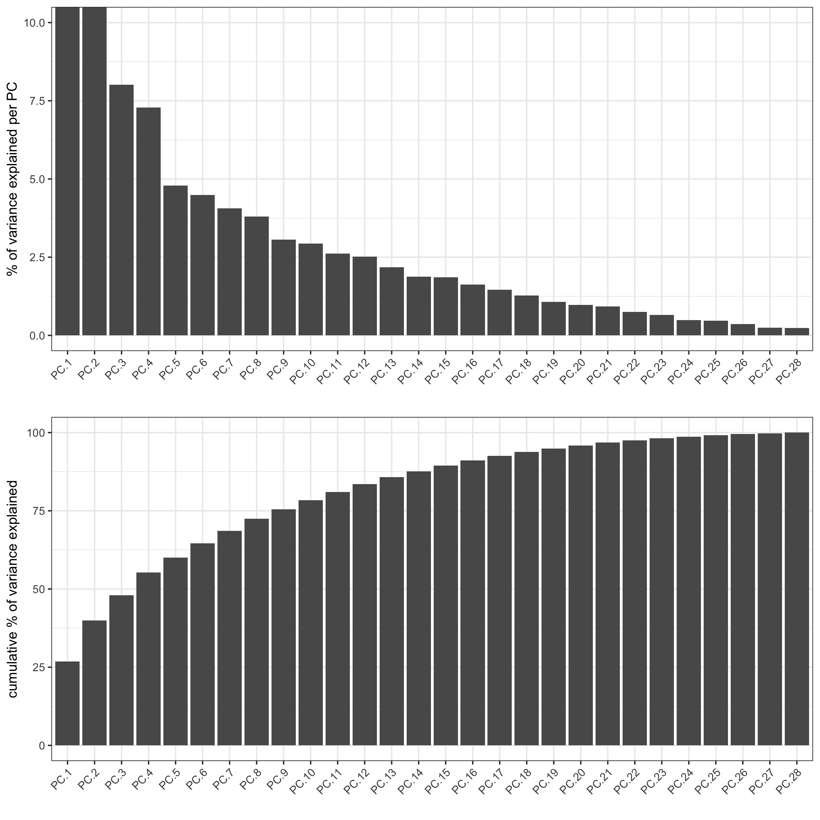
STAR_test <- runUMAP(STAR_test, dimensions_to_use = 1:8, n_components = 3, n_threads = 4)
plotUMAP_3D(gobject = STAR_test,
            save_param = list(save_name = '3_c_UMAP'))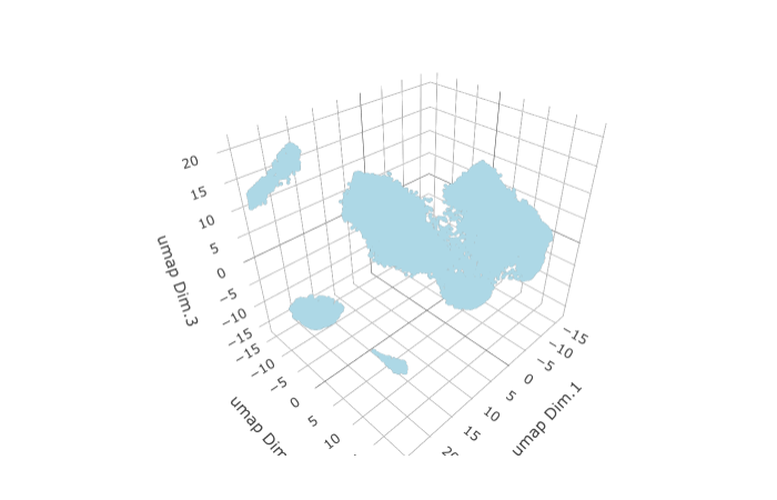
part 4: cluster
## sNN network (default)
STAR_test <- createNearestNetwork(gobject = STAR_test, dimensions_to_use = 1:8, k = 15)

## Leiden clustering
STAR_test <- doLeidenCluster(gobject = STAR_test, resolution = 0.2, n_iterations = 100,
                             name = 'leiden_0.2')

plotUMAP_3D(gobject = STAR_test, cell_color = 'leiden_0.2',show_center_label = F,
            save_param = list(save_name = '4_a_UMAP'))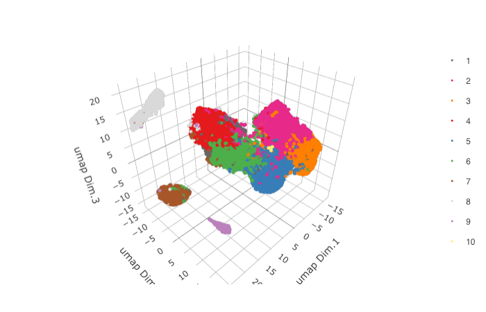
part 5: co-visualize
spatDimPlot3D(gobject = STAR_test,
              cell_color = 'leiden_0.2',
              save_param = list(save_name = '5_a_spatDimPlot'))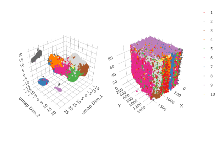
part 6: differential expression
markers = findMarkers_one_vs_all(gobject = STAR_test,
                                 method = 'gini',
                                 expression_values = 'normalized',
                                 cluster_column = 'leiden_0.2',
                                 min_expr_gini_score = 2,
                                 min_det_gini_score = 2,
                                 min_genes = 5, rank_score = 2)
markers[, head(.SD, 2), by = 'cluster']

# violinplot
violinPlot(STAR_test, genes = unique(markers$genes), cluster_column = 'leiden_0.2',
           strip_position = "right", save_param = list(save_name = '6_a_violinplot'))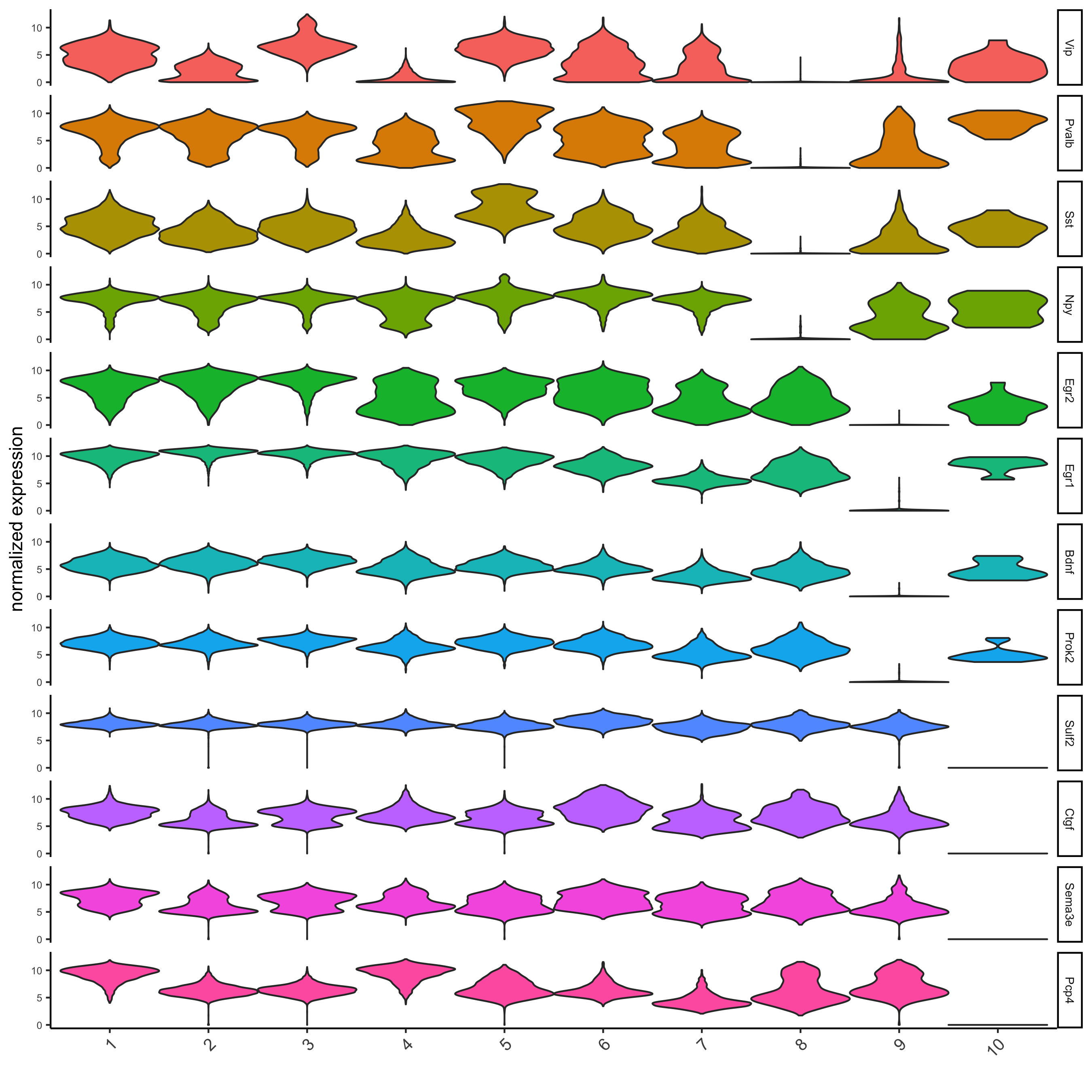
# cluster heatmap
plotMetaDataHeatmap(STAR_test, expression_values = 'scaled',
                    metadata_cols = c('leiden_0.2'),
                    save_param = list(save_name = '6_b_metaheatmap'))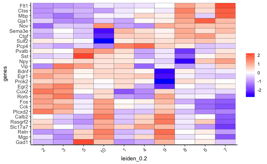
part 7: cell-type annotation
## general cell types
clusters_cell_types_cortex = c('excit','excit','excit', 'inh', 'excit',
                               'other', 'other', 'other', 'inh', 'inh')
names(clusters_cell_types_cortex) = c(1:10)
STAR_test = annotateGiotto(gobject = STAR_test, annotation_vector = clusters_cell_types_cortex,
                           cluster_column = 'leiden_0.2', name = 'general_cell_types')

plotMetaDataHeatmap(STAR_test, expression_values = 'scaled',
                    metadata_cols = c('general_cell_types'),
                    save_param = list(save_name = '7_a_metaheatmap'))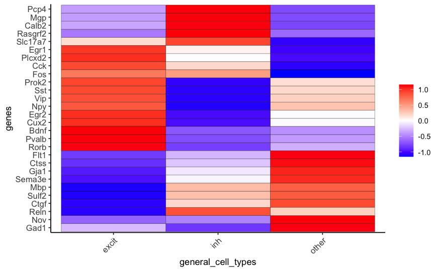
## detailed cell types
clusters_cell_types_cortex = c('L5','L4','L2/3', 'PV', 'L6',
                               'Astro', 'Olig1', 'Olig2', 'Calretinin', 'SST')
names(clusters_cell_types_cortex) = c(1:10)
STAR_test = annotateGiotto(gobject = STAR_test, annotation_vector = clusters_cell_types_cortex,
                           cluster_column = 'leiden_0.2', name = 'cell_types')

plotUMAP_3D(STAR_test, cell_color = 'cell_types', point_size = 1.5,show_center_label = F,
            save_param = list(save_name = '7_b_UMAP'))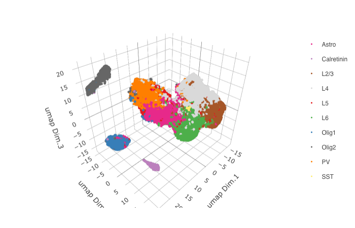
plotMetaDataHeatmap(STAR_test, expression_values = 'scaled',
                    metadata_cols = c('cell_types'),
                    custom_cluster_order = c("Calretinin", "SST", "L4", "L2/3", "PV", "L5", "L6", "Astro", "Olig2", "Olig1"),
                    save_param = list(save_name = '7_c_metaheatmap'))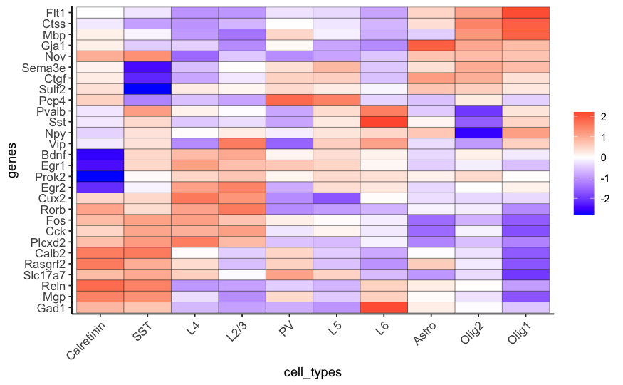
part 8: co-visualize cell types
# create consistent color code
mynames = unique(pDataDT(STAR_test)$cell_types)
mycolorcode = Giotto:::getDistinctColors(n = length(mynames))
names(mycolorcode) = mynames

spatDimPlot3D(gobject = STAR_test,
              cell_color = 'cell_types',show_center_label = F,
              save_param = list(save_name = '8_a_spatdimplot'))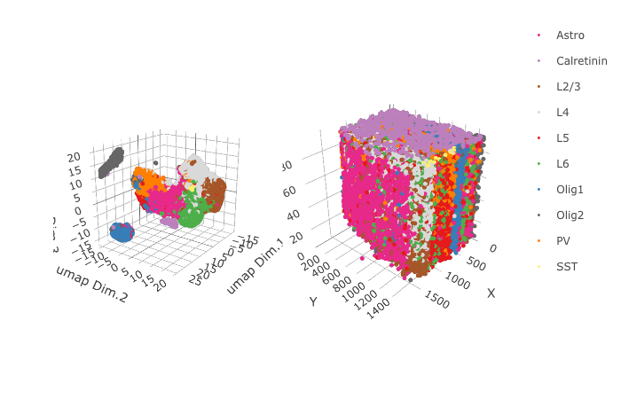
part 9: visualize gene expression
dimGenePlot3D(STAR_test, expression_values = 'scaled',
              genes = "Rorb",
              genes_high_color = 'red', genes_mid_color = 'white', genes_low_color = 'darkblue',
              save_param = list(save_name = '9_a_dimGenePlot'))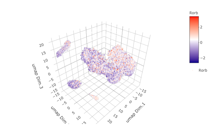
spatGenePlot3D(STAR_test,
               expression_values = 'scaled',
               genes = "Rorb",
               show_other_cells = F,
               genes_high_color = 'red', genes_mid_color = 'white', genes_low_color = 'darkblue',
               save_param = list(save_name = '9_b_spatGenePlot'))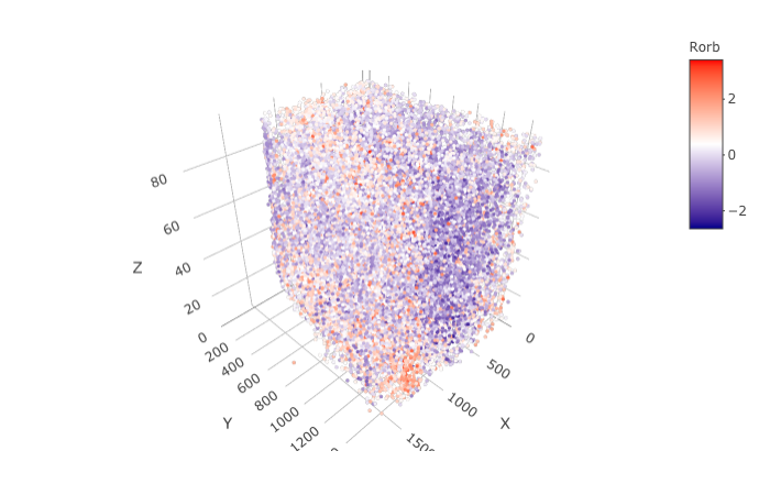
dimGenePlot3D(STAR_test, expression_values = 'scaled',
              genes = "Pcp4",
              genes_high_color = 'red', genes_mid_color = 'white', genes_low_color = 'darkblue',
              save_param = list(save_name = '9_c_dimGenePlot'))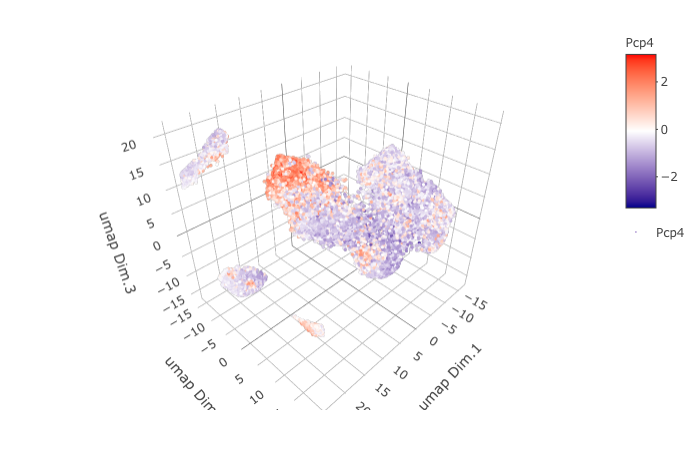
spatGenePlot3D(STAR_test,
               expression_values = 'scaled',
               genes = "Pcp4",
               show_other_cells = F,
               genes_high_color = 'red', genes_mid_color = 'white', genes_low_color = 'darkblue',
               save_param = list(save_name = '9_d_spatGenePlot'))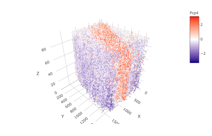
dimGenePlot3D(STAR_test, expression_values = 'scaled',
              genes = "Cux2",
              genes_high_color = 'red', genes_mid_color = 'white', genes_low_color = 'darkblue',
              save_param = list(save_name = '9_e_dimGenePlot'))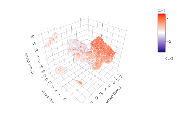
spatGenePlot3D(STAR_test,
               expression_values = 'scaled',
               genes = "Cux2",
               show_other_cells = F,
               genes_high_color = 'red', genes_mid_color = 'white', genes_low_color = 'darkblue',
               save_param = list(save_name = '9_f_spatGenePlot'))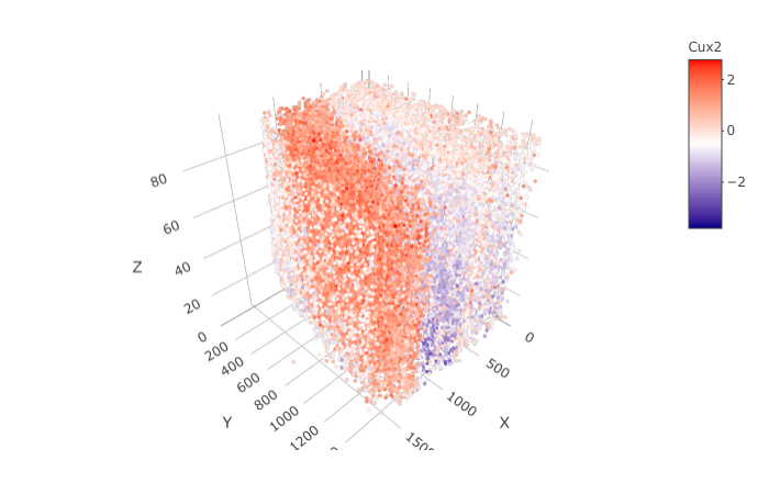
dimGenePlot3D(STAR_test, expression_values = 'scaled',
              genes = "Ctgf",
              genes_high_color = 'red', genes_mid_color = 'white', genes_low_color = 'darkblue',
              save_param = list(save_name = '9_g_dimGenePlot'))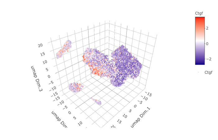
spatGenePlot3D(STAR_test,
               expression_values = 'scaled',
               genes = "Ctgf",
               show_other_cells = F,
               genes_high_color = 'red', genes_mid_color = 'white', genes_low_color = 'darkblue',
               save_param = list(save_name = '9_h_spatGenePlot'))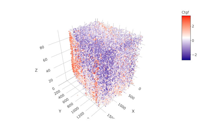
part 10: virtual cross section
STAR_test <- createSpatialNetwork(gobject = STAR_test, delaunay_method = 'delaunayn_geometry')
STAR_test = createCrossSection(STAR_test,method="equation",
                               equation=c(0,1,0,600),
                               extend_ratio = 0.6)
insertCrossSectionSpatPlot3D(STAR_test, cell_color = 'cell_types', axis_scale = 'cube',
                             point_size = 2,
                             cell_color_code = mycolorcode)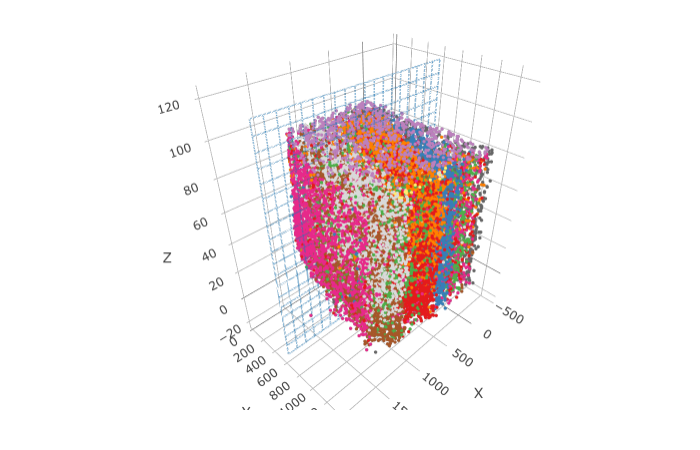
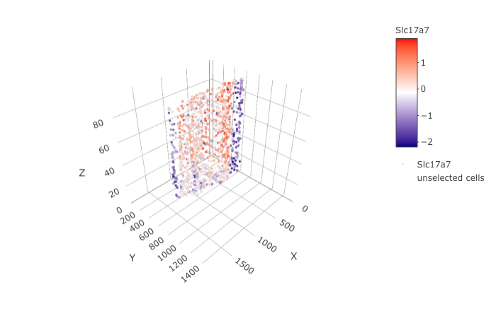
insertCrossSectionGenePlot3D(STAR_test, expression_values = 'scaled', axis_scale = "cube",
                             genes = "Slc17a7")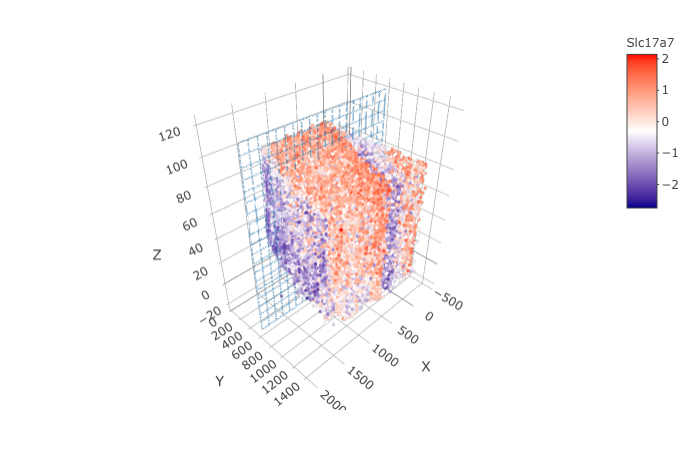
crossSectionPlot(STAR_test,
                 point_size = 2, point_shape = "border",
                 cell_color = "cell_types",cell_color_code = mycolorcode,
                 save_param = list(save_name = '10_a_crossSectionPlot'))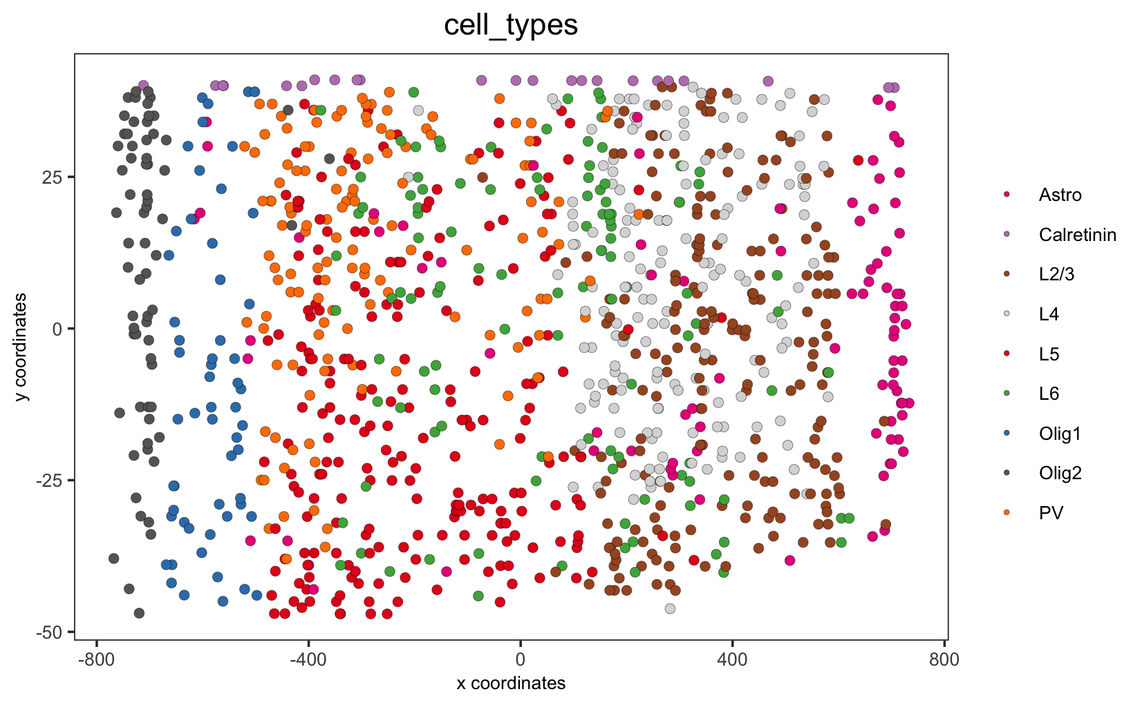
crossSectionPlot3D(STAR_test,
                   point_size = 2, cell_color = "cell_types",
                   cell_color_code = mycolorcode,axis_scale = "cube",
                   save_param = list(save_name = '10_b_crossSectionPlot3D'))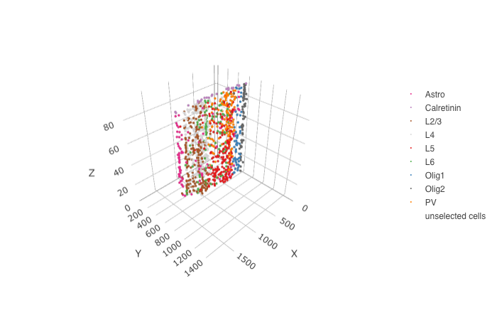
crossSectionGenePlot(STAR_test,
                     genes = "Slc17a7",
                     point_size = 2,point_shape = "border",
                     cow_n_col = 1.5,
                     expression_values = 'scaled',
                     save_param = list(save_name = '10_c_crossSectionGenePlot'))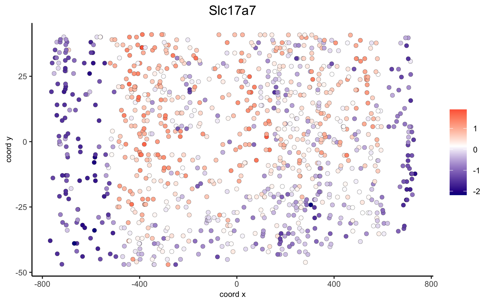
crossSectionGenePlot3D(STAR_test,
                       point_size = 2,
                       genes = c("Slc17a7"),
                       expression_values = 'scaled',
                       save_param = list(save_name = '10_d_crossSectionGenePlot3D'))