Install Python modules
To run this vignette you need to install all the necessary Python modules.
This can be done manually, see https://rubd.github.io/Giotto_site/articles/installation_issues.html#python-manual-installation
This can be done within R using our installation tools (installGiottoEnvironment), see https://rubd.github.io/Giotto_site/articles/tut0_giotto_environment.html for more information.
(optional) set giotto instructions
# to automatically save figures in save_dir set save_plot to TRUE
temp_dir = getwd()
temp_dir = '~/Temp/'
myinstructions = createGiottoInstructions(save_dir = temp_dir,
                                          save_plot = TRUE,
                                          show_plot = FALSE)
1. Create a Giotto object
minimum requirements:
- matrix with expression information (or path to)
- x,y(,z) coordinates for cells or spots (or path to)
# giotto object
expr_path = system.file("extdata", "seqfish_field_expr.txt.gz", package = 'Giotto')
loc_path = system.file("extdata", "seqfish_field_locs.txt", package = 'Giotto')
seqfish_mini <- createGiottoObject(raw_exprs = expr_path,
                                   spatial_locs = loc_path,
                                   instructions = myinstructions)
How to work with Giotto instructions that are part of your Giotto
object:
- show the instructions associated with your Giotto object with
showGiottoInstructions
- change one or more instructions with
changeGiottoInstructions
- replace all instructions at once with
replaceGiottoInstructions
- read or get a specific giotto instruction with
readGiottoInstructions
Of note, the python path can only be set once in an R session. See the
reticulate package for more information.
# show instructions associated with giotto object (seqfish_mini)
showGiottoInstructions(seqfish_mini)
2. processing steps
- filter genes and cells based on detection frequencies
- normalize expression matrix (log transformation, scaling factor and/or z-scores)
- add cell and gene statistics (optional)
- adjust expression matrix for technical covariates or batches (optional). These results will be stored in the custom slot.
seqfish_mini <- filterGiotto(gobject = seqfish_mini,
                             expression_threshold = 0.5,
                             gene_det_in_min_cells = 20,
                             min_det_genes_per_cell = 0)
seqfish_mini <- normalizeGiotto(gobject = seqfish_mini, scalefactor = 6000, verbose = T)
seqfish_mini <- addStatistics(gobject = seqfish_mini)
seqfish_mini <- adjustGiottoMatrix(gobject = seqfish_mini,
                                   expression_values = c('normalized'),
                                   covariate_columns = c('nr_genes', 'total_expr'))
3. dimension reduction
- identify highly variable genes (HVG)
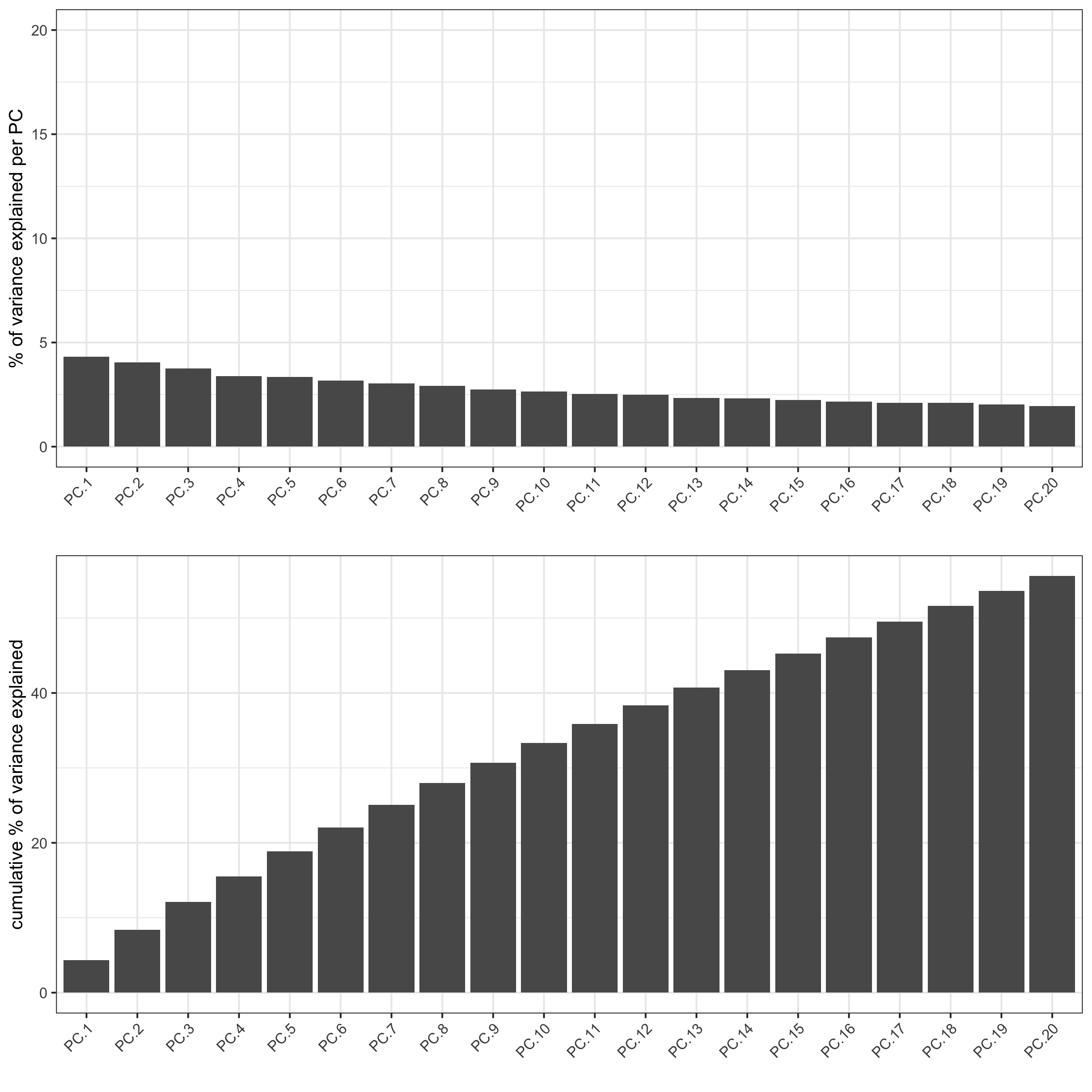
- perform PCA
- identify number of significant prinicipal components (PCs)
- run UMAP and/or TSNE on PCs (or directly on matrix)
seqfish_mini <- calculateHVG(gobject = seqfish_mini)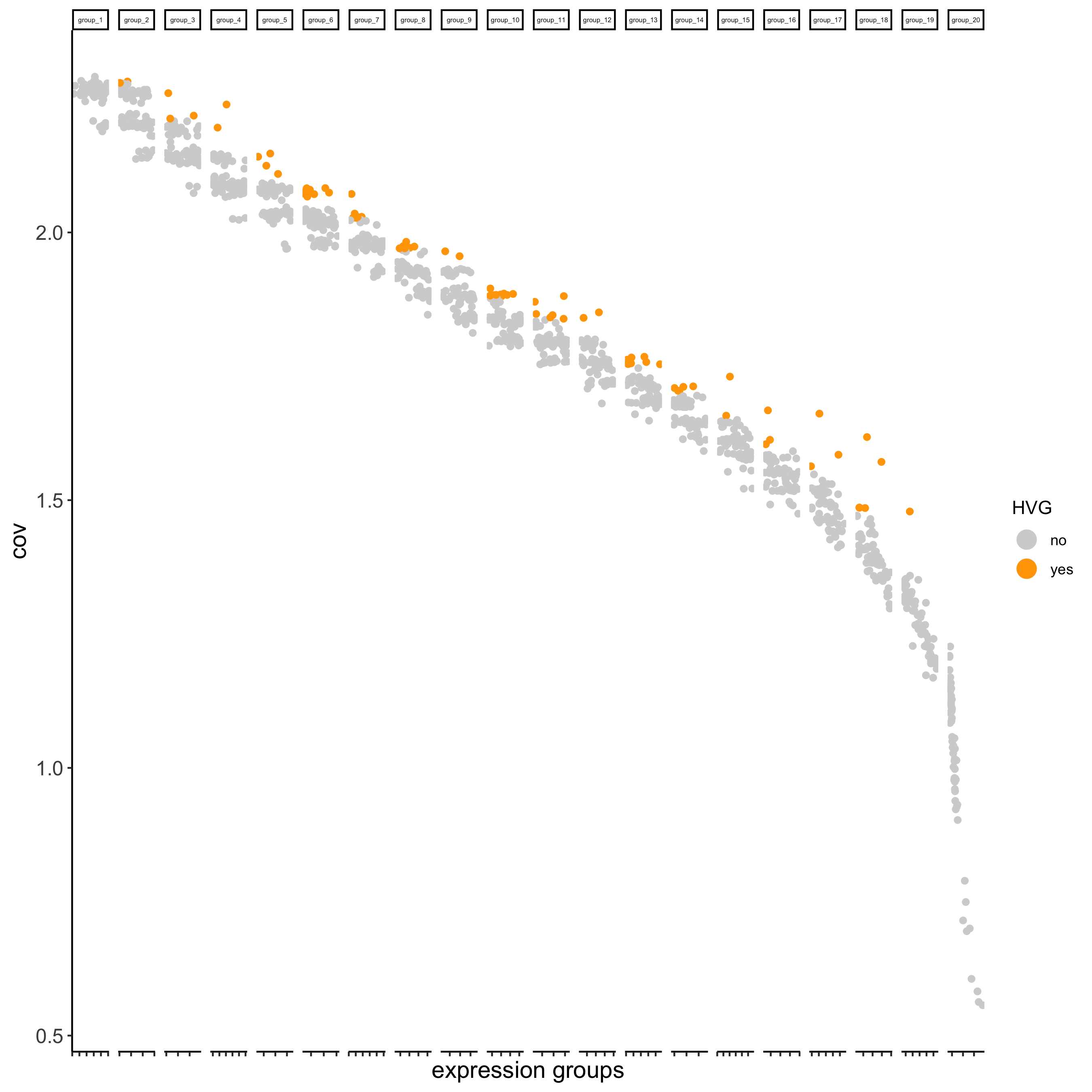
jackstrawPlot(seqfish_mini, ncp = 20)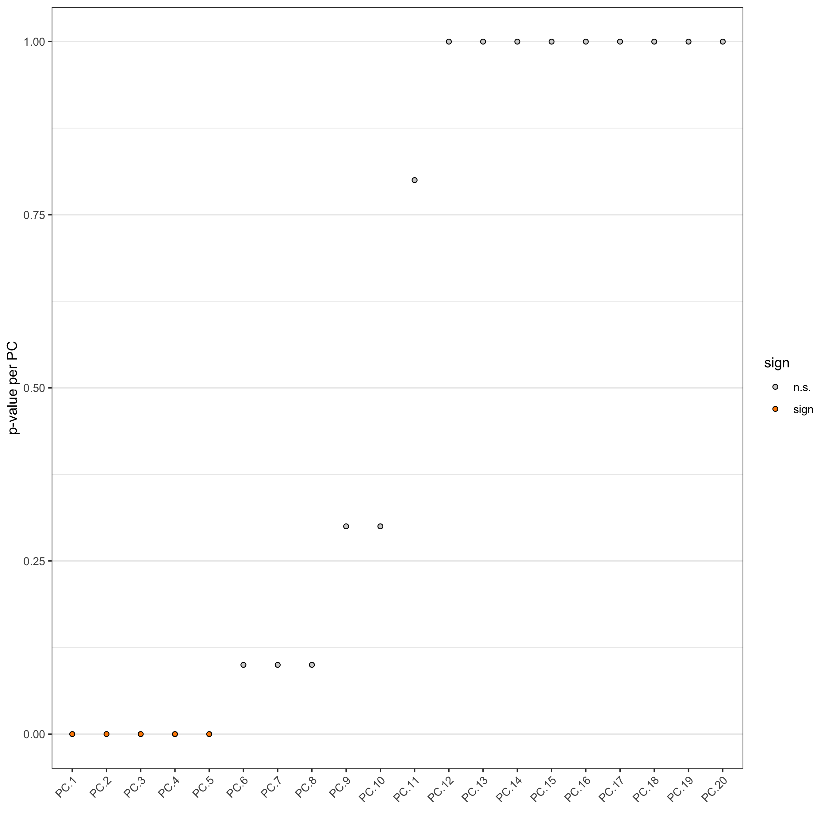
plotPCA(seqfish_mini)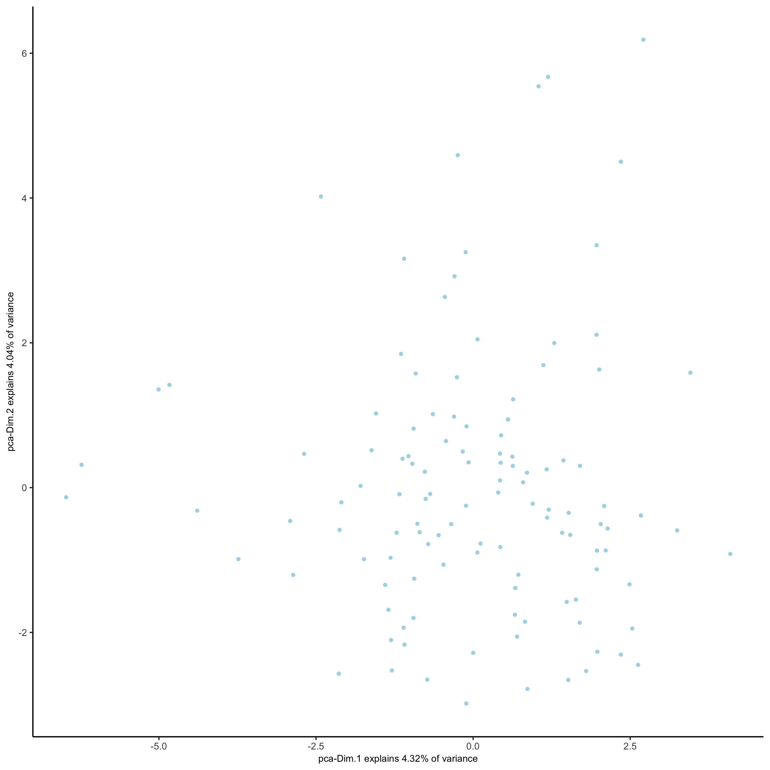
seqfish_mini <- runUMAP(seqfish_mini, dimensions_to_use = 1:5, n_threads = 2)
plotUMAP(gobject = seqfish_mini)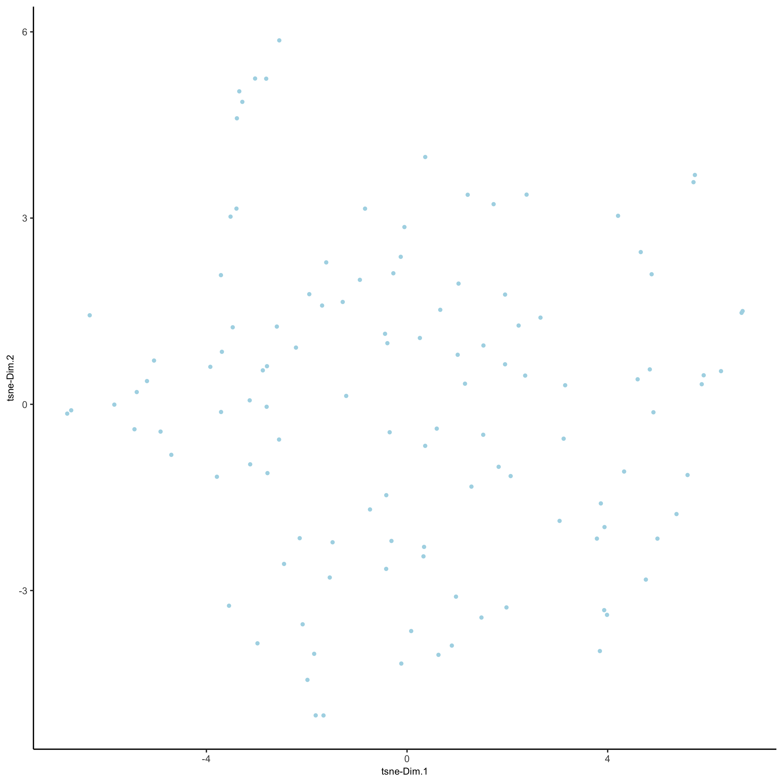
4. clustering
- create a shared (default) nearest network in PCA space (or directly
on matrix)
- cluster on nearest network with Leiden or Louvan (kmeans and hclust are alternatives)
seqfish_mini <- createNearestNetwork(gobject = seqfish_mini, dimensions_to_use = 1:5, k = 5)
seqfish_mini <- doLeidenCluster(gobject = seqfish_mini, resolution = 0.4, n_iterations = 1000)

# visualize UMAP cluster results
plotUMAP(gobject = seqfish_mini, cell_color = 'leiden_clus',
         show_NN_network = T, point_size = 2.5)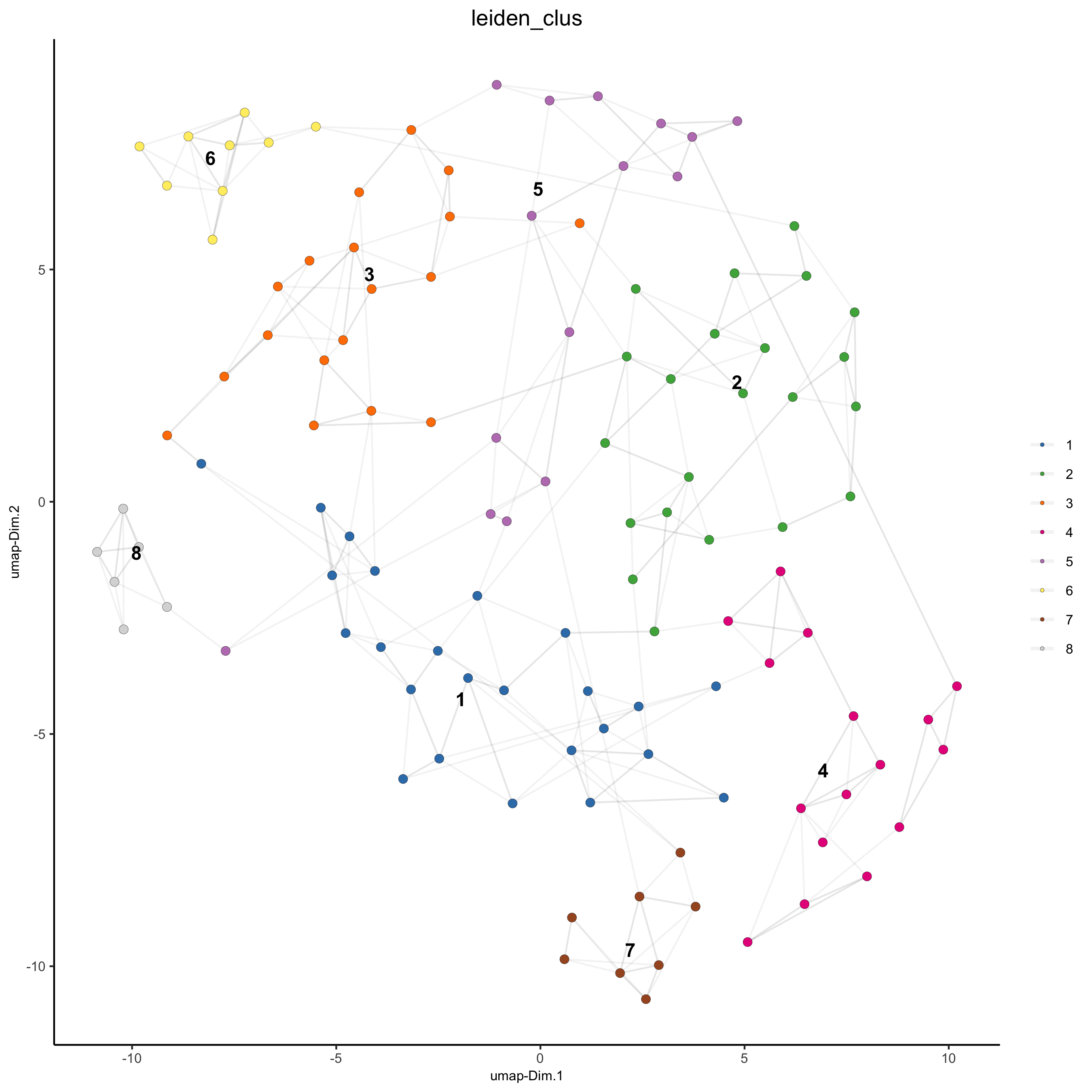
# visualize UMAP and spatial results
spatDimPlot(gobject = seqfish_mini, cell_color = 'leiden_clus', spat_point_shape = 'voronoi')

# heatmap and dendrogram
showClusterHeatmap(gobject = seqfish_mini, cluster_column = 'leiden_clus')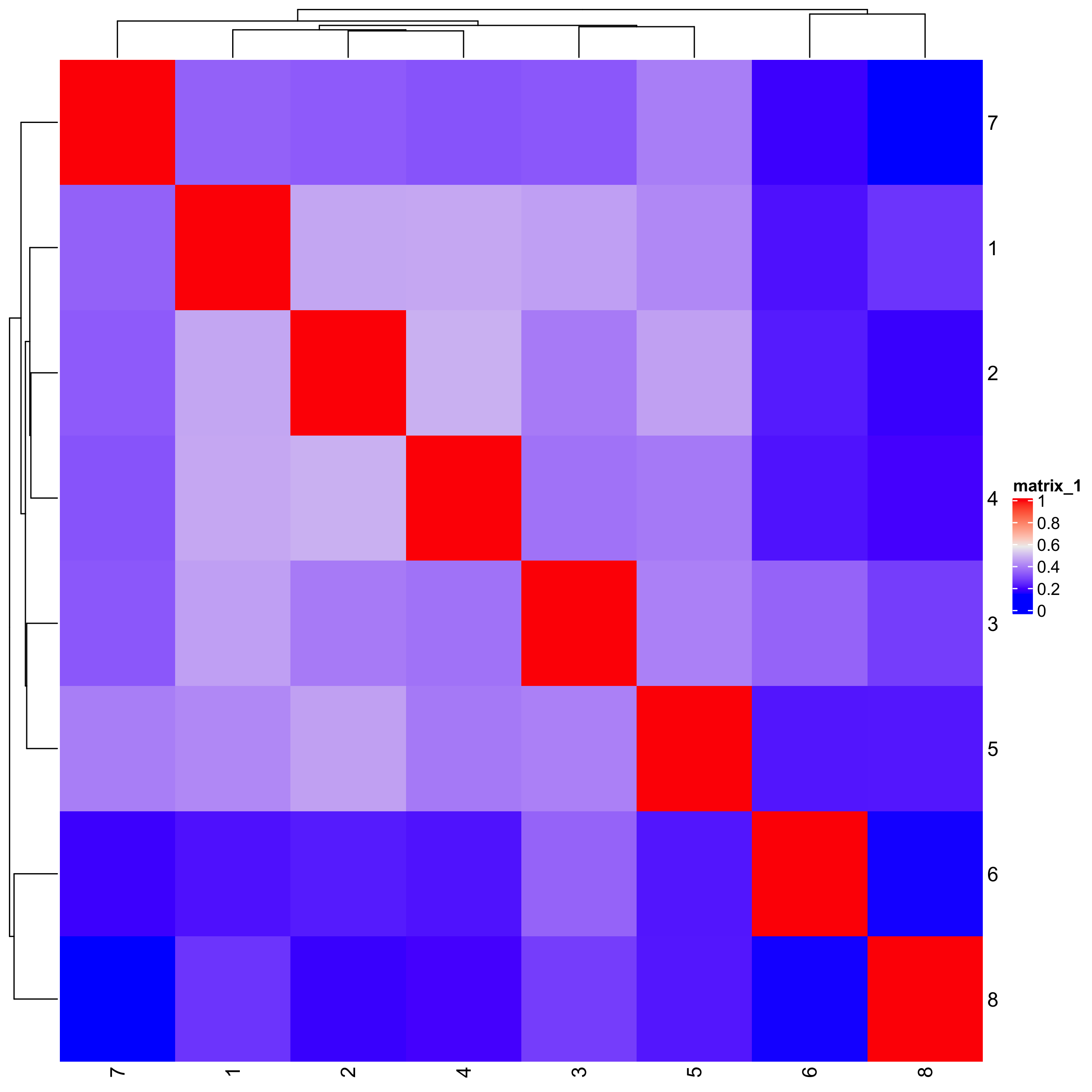
showClusterDendrogram(seqfish_mini, h = 0.5, rotate = T, cluster_column = 'leiden_clus')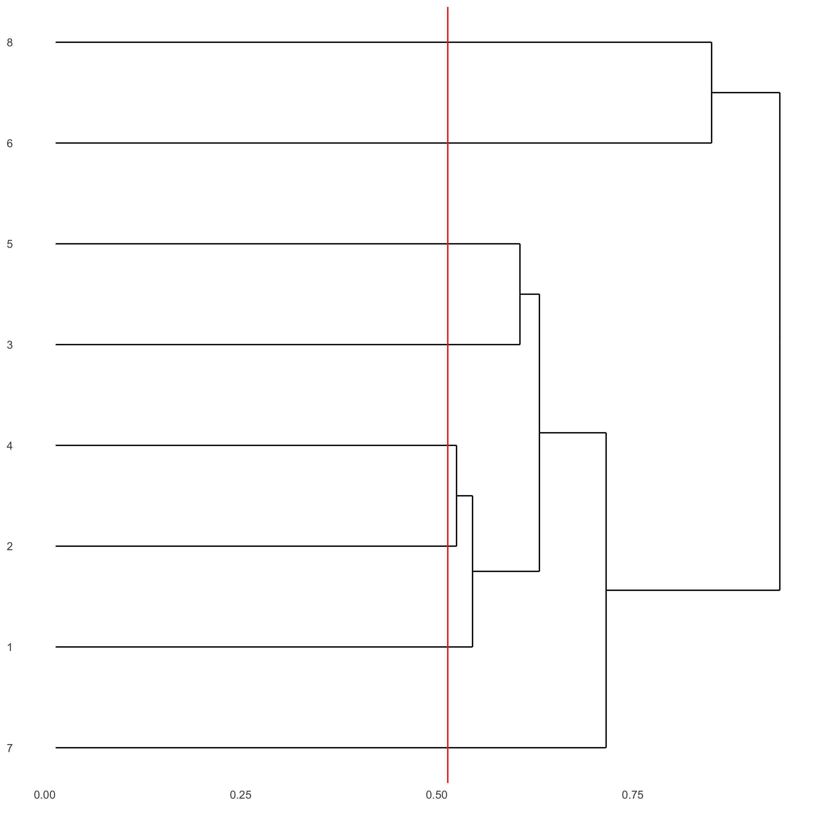
5. differential expression
gini_markers = findMarkers_one_vs_all(gobject = seqfish_mini,
                                                  method = 'gini',
                                                  expression_values = 'normalized',
                                                  cluster_column = 'leiden_clus',
                                                  min_genes = 20,
                                                  min_expr_gini_score = 0.5,
                                                  min_det_gini_score = 0.5)

# get top 2 genes per cluster and visualize with violinplot
topgenes_gini = gini_markers[, head(.SD, 2), by = 'cluster']
violinPlot(seqfish_mini, genes = topgenes_gini$genes, cluster_column = 'leiden_clus')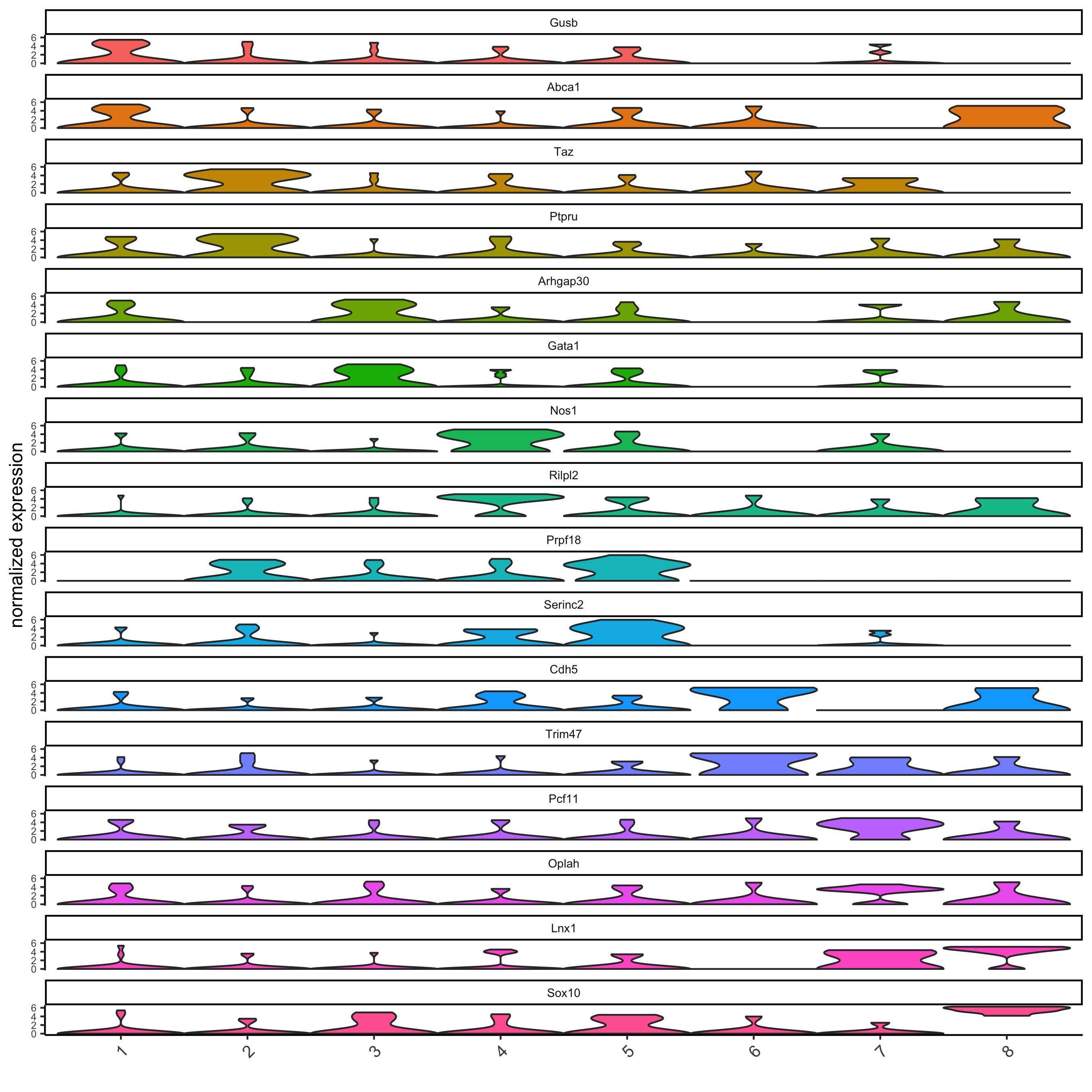
# get top 6 genes per cluster and visualize with heatmap
topgenes_gini2 = gini_markers[, head(.SD, 6), by = 'cluster']
plotMetaDataHeatmap(seqfish_mini, selected_genes = topgenes_gini2$genes,
                    metadata_cols = c('leiden_clus'))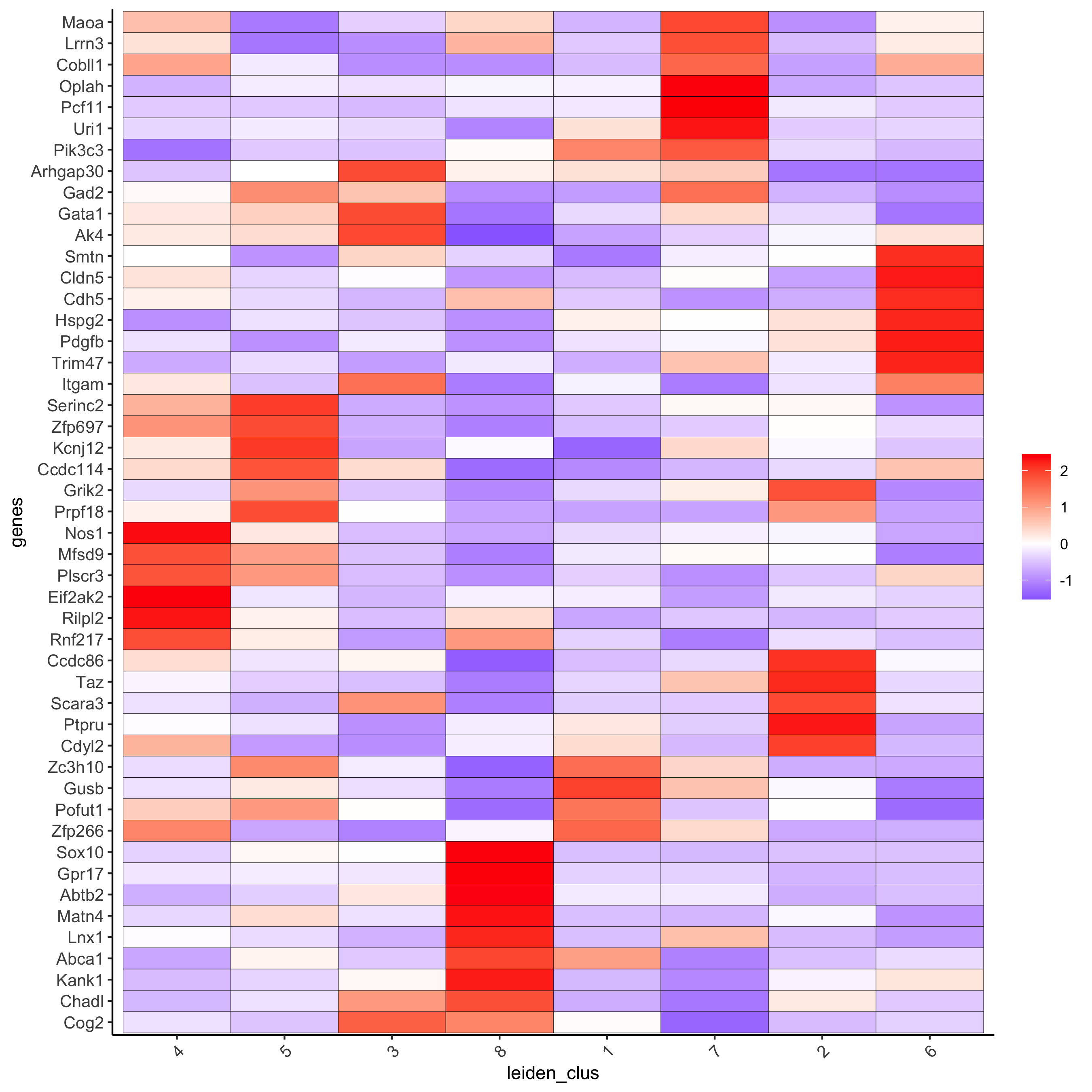
6. cell type annotation
clusters_cell_types = c('cell A', 'cell B', 'cell C', 'cell D',
                        'cell E', 'cell F', 'cell G')
names(clusters_cell_types) = 1:7
seqfish_mini = annotateGiotto(gobject = seqfish_mini,
                              annotation_vector = clusters_cell_types,
                              cluster_column = 'leiden_clus',
                              name = 'cell_types')
# check new cell metadata
pDataDT(seqfish_mini)

# visualize annotations
spatDimPlot(gobject = seqfish_mini, cell_color = 'cell_types',
            spat_point_size = 3, dim_point_size = 3)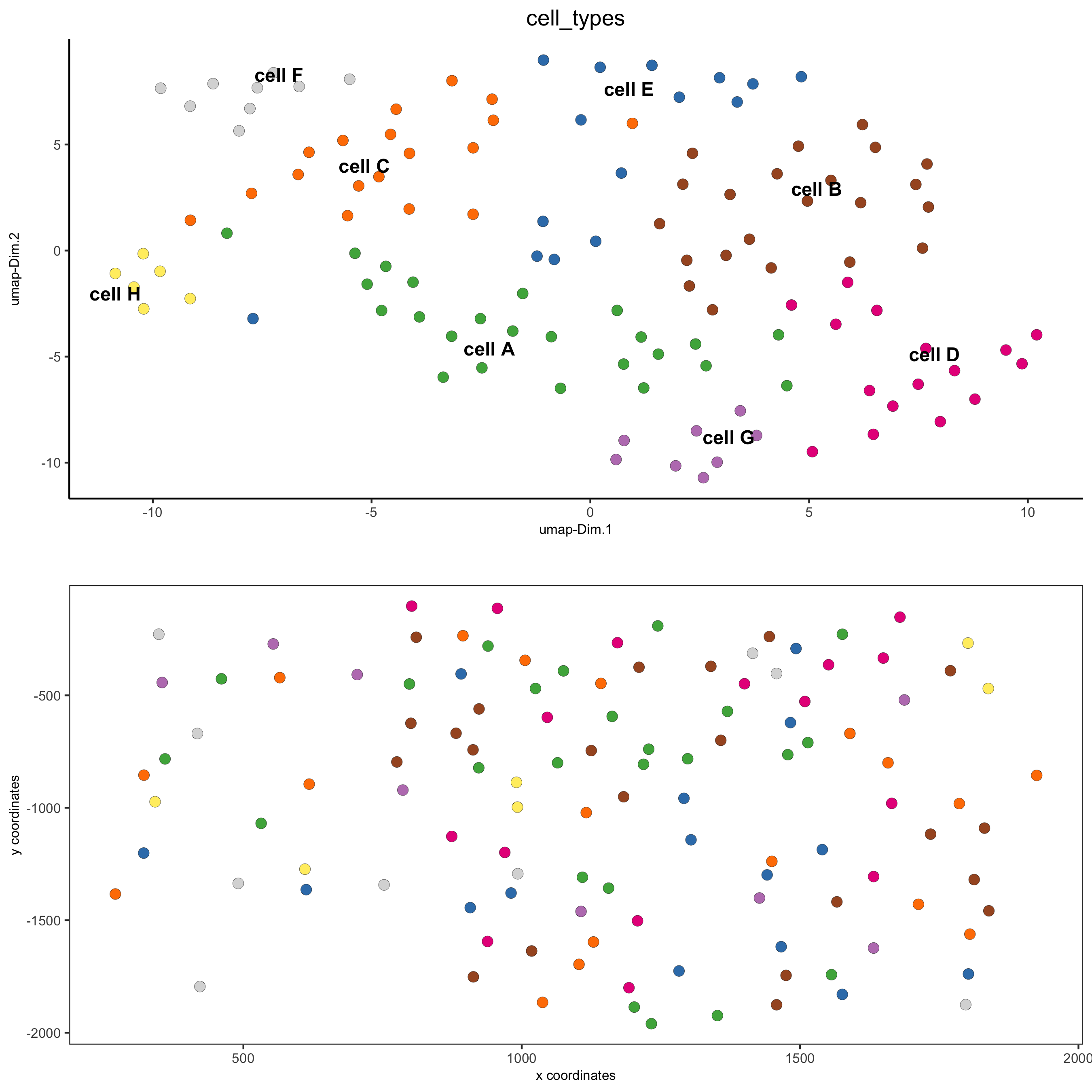
7. spatial grid
Create a grid based on defined stepsizes in the x,y(,z) axes.
seqfish_mini <- createSpatialGrid(gobject = seqfish_mini,
                              sdimx_stepsize = 300,
                              sdimy_stepsize = 300,
                              minimum_padding = 50)
showGrids(seqfish_mini)

# visualize grid
spatPlot(gobject = seqfish_mini, show_grid = T, point_size = 1.5)
8. spatial network
- visualize information about the default Delaunay network
- create a spatial Delaunay network (default)
- create a spatial kNN network
plotStatDelaunayNetwork(gobject = seqfish_mini, maximum_distance = 400)
seqfish_mini = createSpatialNetwork(gobject = seqfish_mini, minimum_k = 2,
                                    maximum_distance_delaunay = 400)
seqfish_mini = createSpatialNetwork(gobject = seqfish_mini, minimum_k = 2,
                                    method = 'kNN', k = 10)
showNetworks(seqfish_mini)

# visualize the two different spatial networks
spatPlot(gobject = seqfish_mini, show_network = T,
         network_color = 'blue', spatial_network_name = 'Delaunay_network',
         point_size = 2.5, cell_color = 'leiden_clus')

spatPlot(gobject = seqfish_mini, show_network = T,
         network_color = 'blue', spatial_network_name = 'kNN_network',
         point_size = 2.5, cell_color = 'leiden_clus')
9. spatial genes
Identify spatial genes with 3 different methods:
- binSpect with kmeans binarization (default)
- binSpect with rank binarization
- silhouetteRank
Visualize top 4 genes per method.
km_spatialgenes = binSpect(seqfish_mini)
spatGenePlot(seqfish_mini, expression_values = 'scaled',
             genes = km_spatialgenes[1:4]$genes,
             point_shape = 'border', point_border_stroke = 0.1,
             show_network = F, network_color = 'lightgrey', point_size = 2.5,
             cow_n_col = 2)

rank_spatialgenes = binSpect(seqfish_mini, bin_method = 'rank')
spatGenePlot(seqfish_mini, expression_values = 'scaled',
             genes = rank_spatialgenes[1:4]$genes,
             point_shape = 'border', point_border_stroke = 0.1,
             show_network = F, network_color = 'lightgrey', point_size = 2.5,
             cow_n_col = 2)
silh_spatialgenes = silhouetteRank(gobject = seqfish_mini) # TODO: suppress print output
spatGenePlot(seqfish_mini, expression_values = 'scaled',
             genes = silh_spatialgenes[1:4]$genes,
             point_shape = 'border', point_border_stroke = 0.1,
             show_network = F, network_color = 'lightgrey', point_size = 2.5,
             cow_n_col = 2)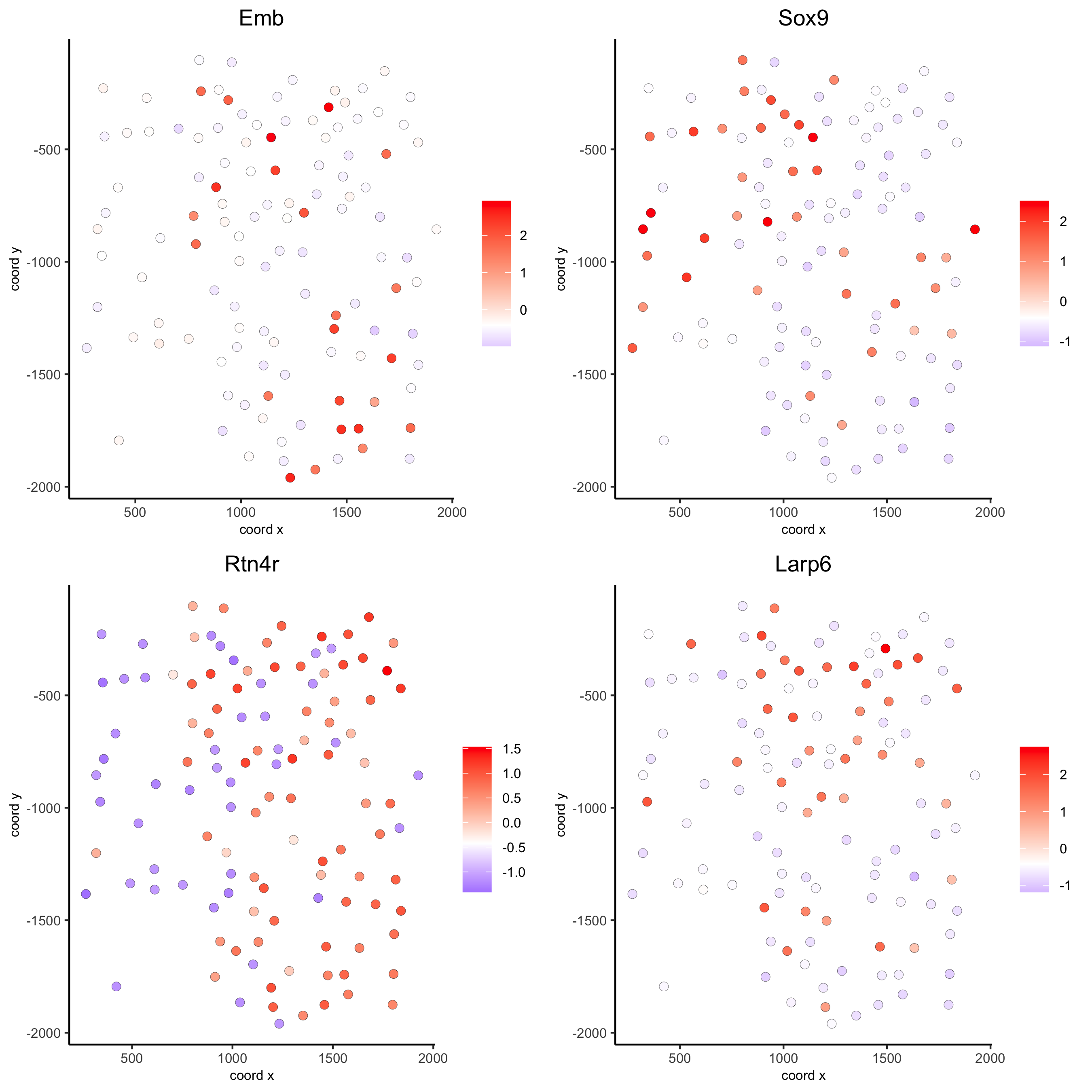
10. spatial co-expression patterns
Identify robust spatial co-expression patterns using the spatial
network or grid and a subset of individual spatial genes.
1. calculate spatial correlation scores
2. cluster correlation scores
# 1. calculate spatial correlation scores
ext_spatial_genes = km_spatialgenes[1:500]$genes
spat_cor_netw_DT = detectSpatialCorGenes(seqfish_mini,
                                         method = 'network',
                                         spatial_network_name = 'Delaunay_network',
                                         subset_genes = ext_spatial_genes)

# 2. cluster correlation scores
spat_cor_netw_DT = clusterSpatialCorGenes(spat_cor_netw_DT,
                                          name = 'spat_netw_clus', k = 8)
heatmSpatialCorGenes(seqfish_mini, spatCorObject = spat_cor_netw_DT,
                     use_clus_name = 'spat_netw_clus')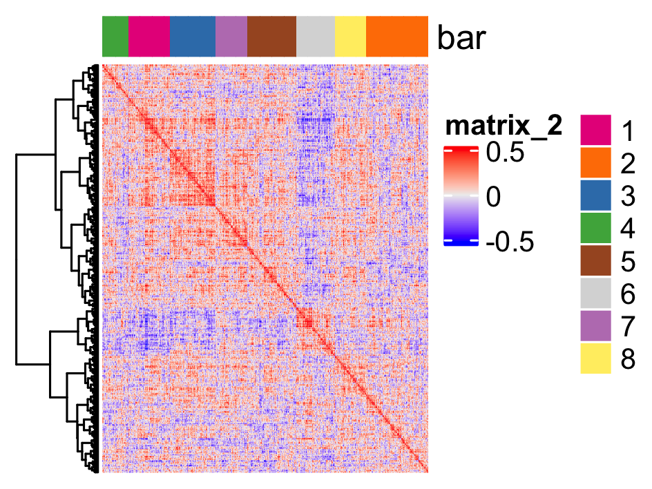
netw_ranks = rankSpatialCorGroups(seqfish_mini,
                                  spatCorObject = spat_cor_netw_DT,
                                  use_clus_name = 'spat_netw_clus')
top_netw_spat_cluster = showSpatialCorGenes(spat_cor_netw_DT,
                                            use_clus_name = 'spat_netw_clus',
                                            selected_clusters = 6,
                                            show_top_genes = 1)

cluster_genes_DT = showSpatialCorGenes(spat_cor_netw_DT,
                                       use_clus_name = 'spat_netw_clus',
                                       show_top_genes = 1)
cluster_genes = cluster_genes_DT$clus; names(cluster_genes) = cluster_genes_DT$gene_ID

seqfish_mini = createMetagenes(seqfish_mini, gene_clusters = cluster_genes, name = 'cluster_metagene')
spatCellPlot(seqfish_mini,
             spat_enr_names = 'cluster_metagene',
             cell_annotation_values = netw_ranks$clusters,
             point_size = 1.5, cow_n_col = 3)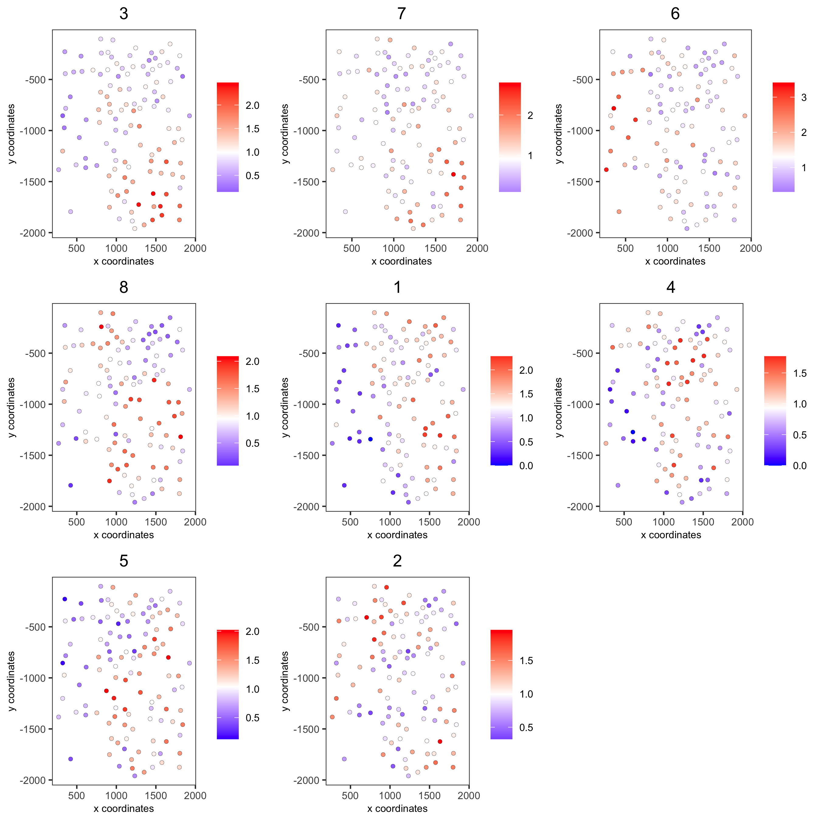
11. spatial HMRF domains
hmrf_folder = paste0(temp_dir,'/','11_HMRF/')
if(!file.exists(hmrf_folder)) dir.create(hmrf_folder, recursive = T)

# perform hmrf
my_spatial_genes = km_spatialgenes[1:100]$genes
HMRF_spatial_genes = doHMRF(gobject = seqfish_mini,
                            expression_values = 'scaled',
                            spatial_genes = my_spatial_genes,
                            spatial_network_name = 'Delaunay_network',
                            k = 9,
                            betas = c(28,2,2),
                            output_folder = paste0(hmrf_folder, '/', 'Spatial_genes/SG_top100_k9_scaled'))

# check and select hmrf
for(i in seq(28, 30, by = 2)) {
  viewHMRFresults2D(gobject = seqfish_mini,
                    HMRFoutput = HMRF_spatial_genes,
                    k = 9, betas_to_view = i,
                    point_size = 2)
}

seqfish_mini = addHMRF(gobject = seqfish_mini,
                  HMRFoutput = HMRF_spatial_genes,
                  k = 9, betas_to_add = c(28),
                  hmrf_name = 'HMRF')

# visualize selected hmrf result
giotto_colors = Giotto:::getDistinctColors(9)
names(giotto_colors) = 1:9
spatPlot(gobject = seqfish_mini, cell_color = 'HMRF_k9_b.28',
         point_size = 3, coord_fix_ratio = 1, cell_color_code = giotto_colors)
12. cell neighborhood: cell-type/cell-type interactions
set.seed(seed = 2841)
cell_proximities = cellProximityEnrichment(gobject = seqfish_mini,
                                           cluster_column = 'cell_types',
                                           spatial_network_name = 'Delaunay_network',
                                           adjust_method = 'fdr',
                                           number_of_simulations = 1000)
# barplot
cellProximityBarplot(gobject = seqfish_mini,
                     CPscore = cell_proximities,
                     min_orig_ints = 5, min_sim_ints = 5)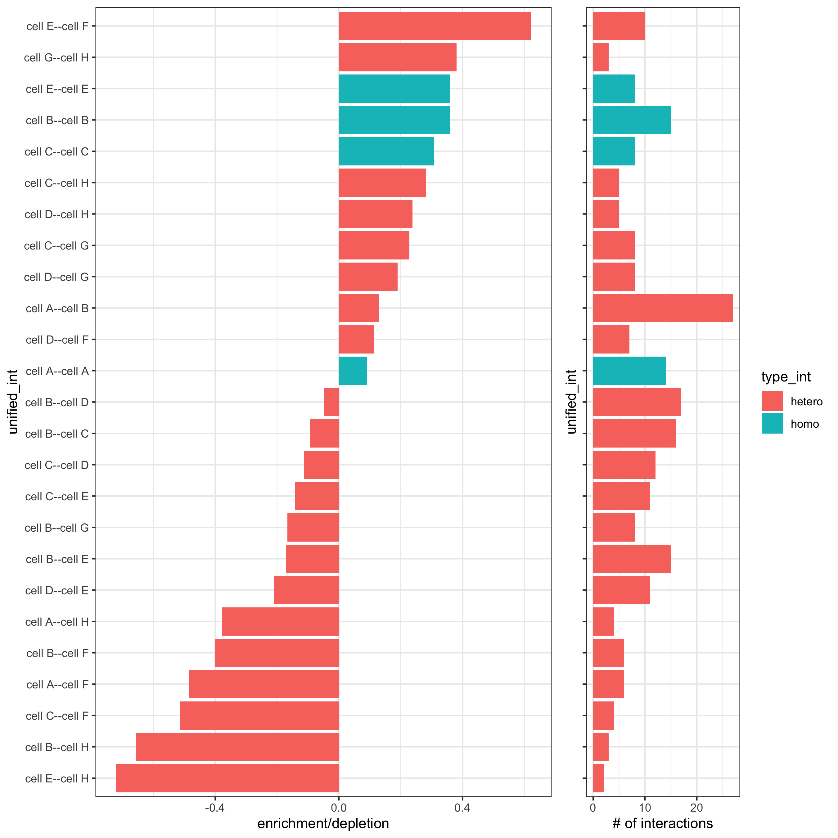
## heatmap
cellProximityHeatmap(gobject = seqfish_mini, CPscore = cell_proximities,
                     order_cell_types = T, scale = T,
                     color_breaks = c(-1.5, 0, 1.5),
                     color_names = c('blue', 'white', 'red'))
# network
cellProximityNetwork(gobject = seqfish_mini, CPscore = cell_proximities,
                     remove_self_edges = T, only_show_enrichment_edges = T)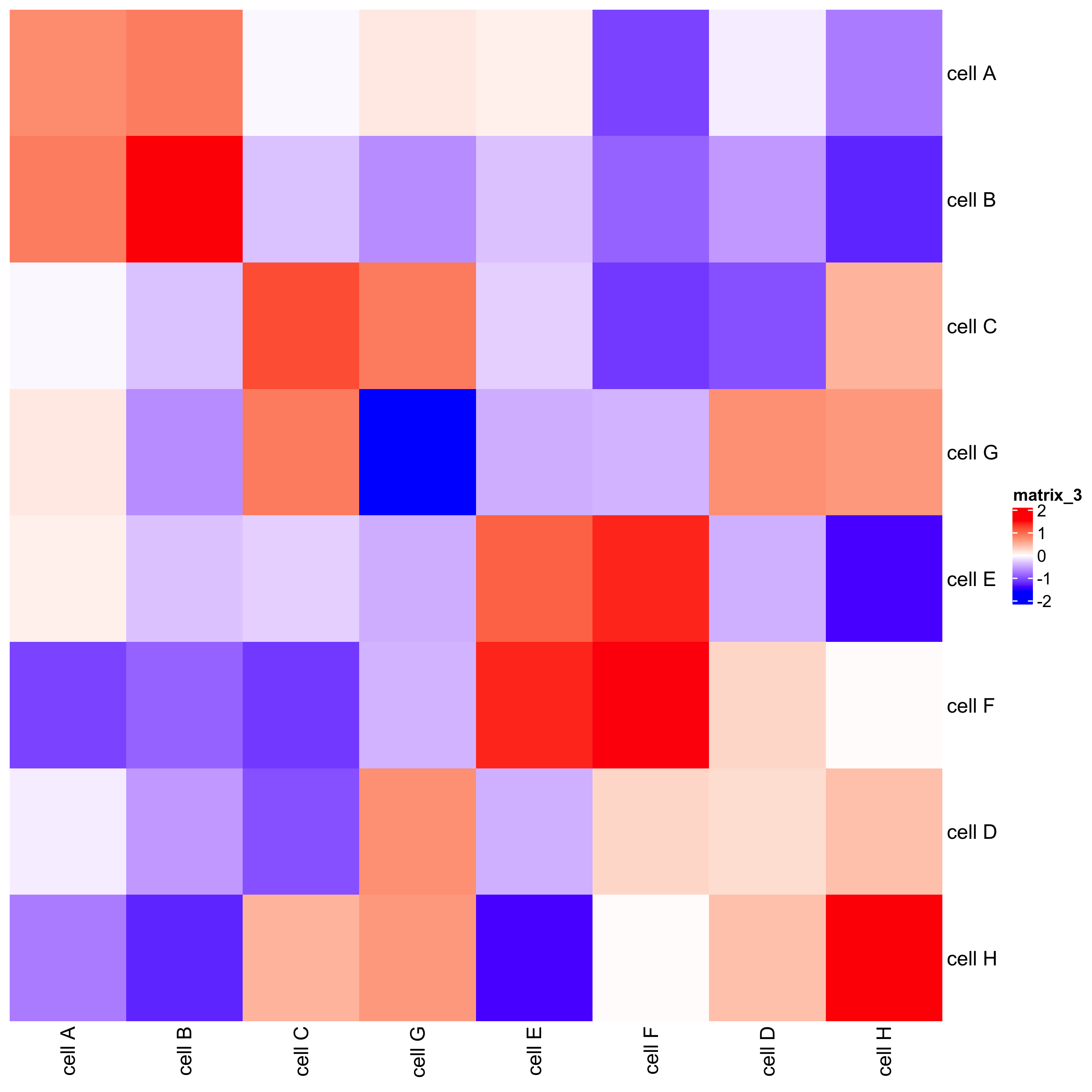
# network with self-edges
cellProximityNetwork(gobject = seqfish_mini, CPscore = cell_proximities,
                     remove_self_edges = F, self_loop_strength = 0.3,
                     only_show_enrichment_edges = F,
                     rescale_edge_weights = T,
                     node_size = 8,
                     edge_weight_range_depletion = c(1, 2),
                     edge_weight_range_enrichment = c(2,5))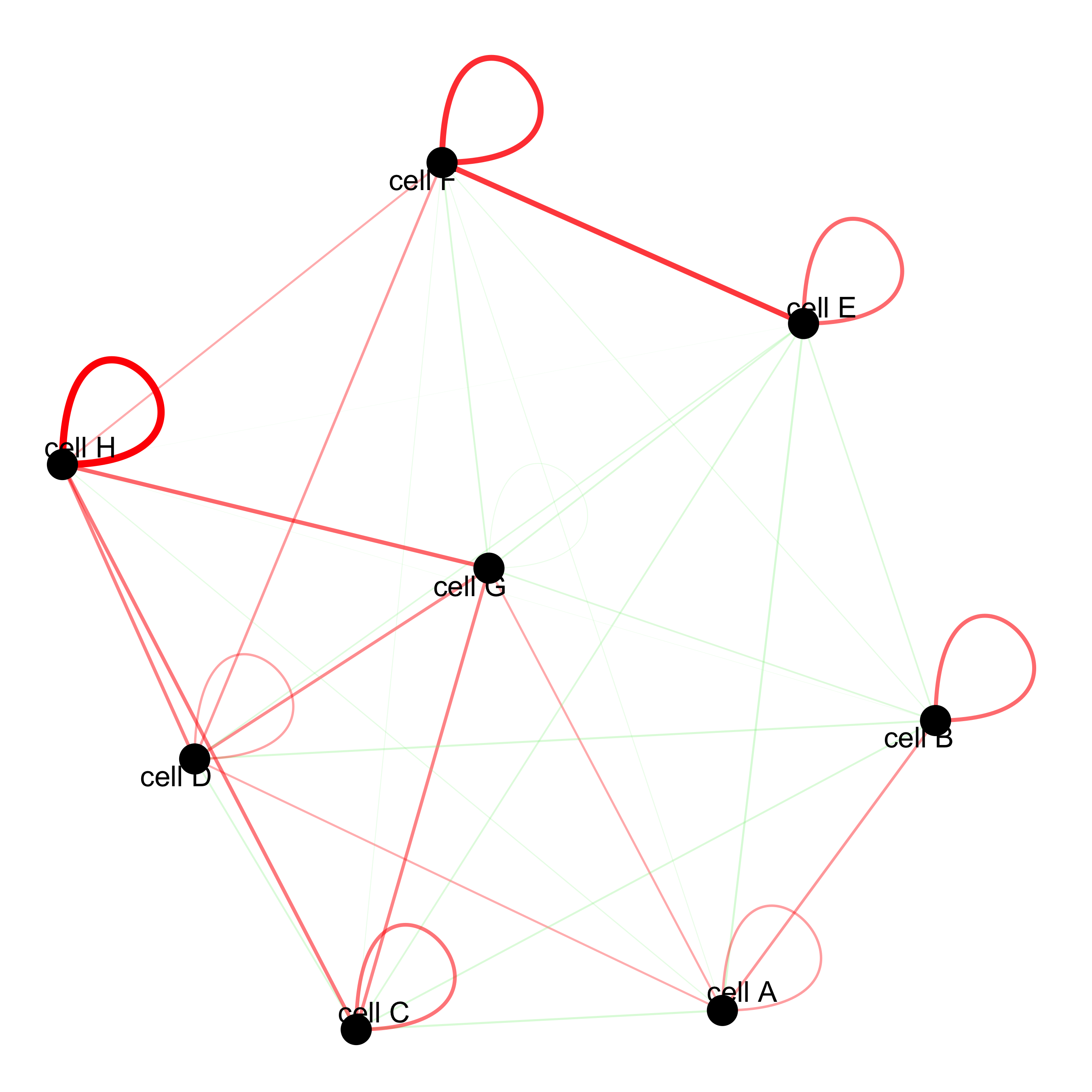
visualization of specific cell types
# Option 1
spec_interaction = "cell D--cell F"
cellProximitySpatPlot2D(gobject = seqfish_mini,
                        interaction_name = spec_interaction,
                        show_network = T,
                        cluster_column = 'cell_types',
                        cell_color = 'cell_types',
                        cell_color_code = c('cell D' = 'lightblue', 'cell F' = 'red'),
                        point_size_select = 4, point_size_other = 2)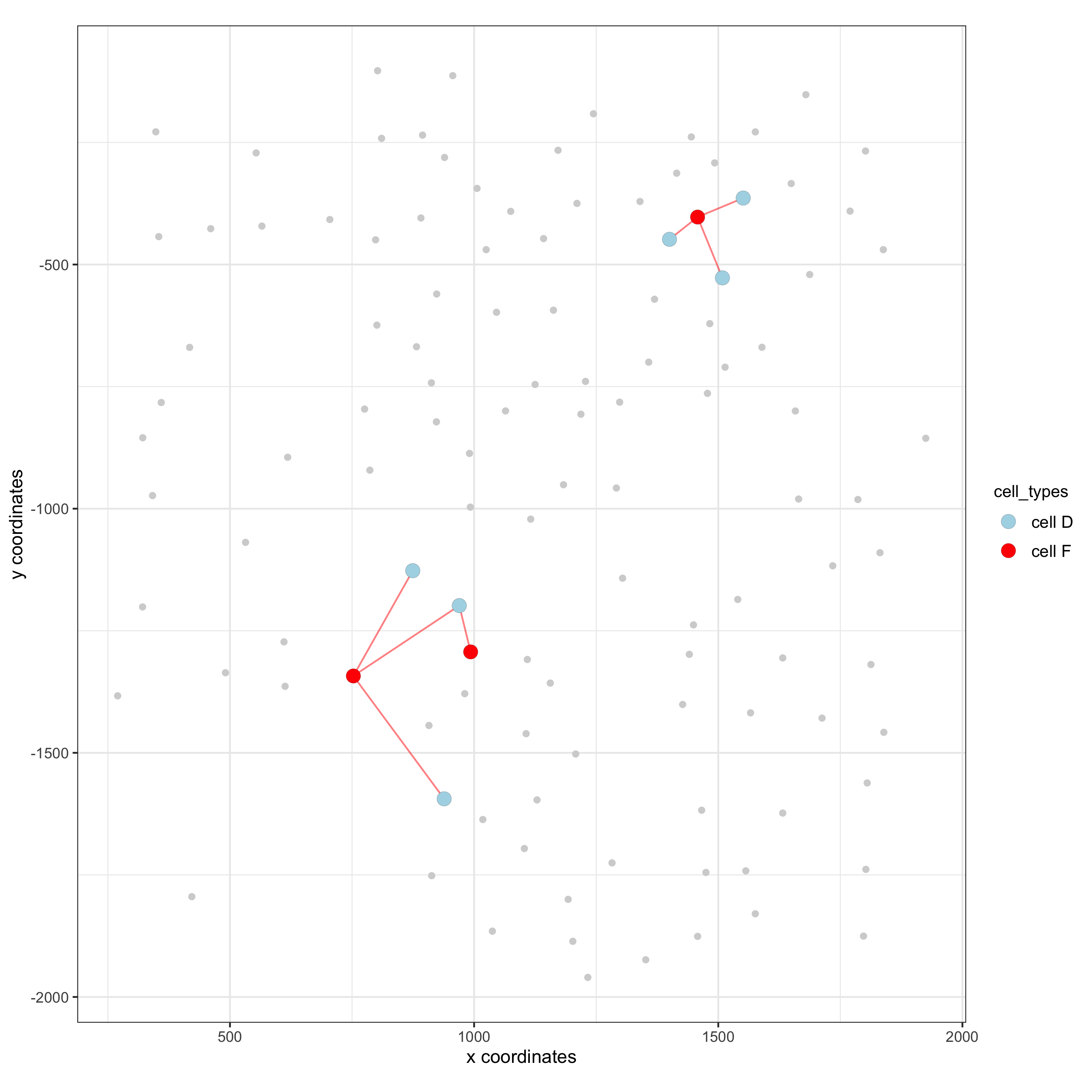
# Option 2: create additional metadata
seqfish_mini = addCellIntMetadata(seqfish_mini,
                             spatial_network = 'Delaunay_network',
                             cluster_column = 'cell_types',
                             cell_interaction = spec_interaction,
                             name = 'D_F_interactions')
spatPlot(seqfish_mini, cell_color = 'D_F_interactions', legend_symbol_size = 3,
         select_cell_groups =  c('other_cell D', 'other_cell F', 'select_cell D', 'select_cell F'))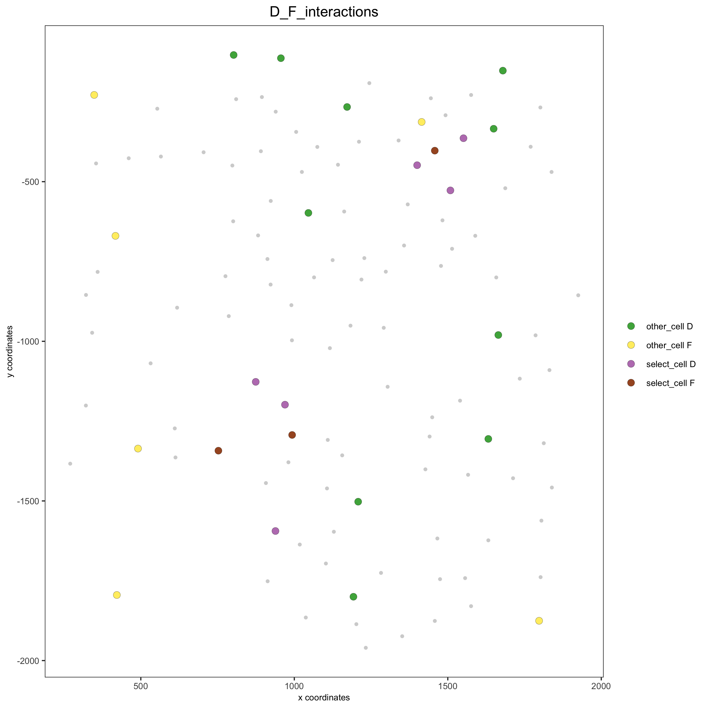
13. cell neighborhood: interaction changed genes
## select top 25th highest expressing genes
gene_metadata = fDataDT(seqfish_mini)
plot(gene_metadata$nr_cells, gene_metadata$mean_expr)
plot(gene_metadata$nr_cells, gene_metadata$mean_expr_det)

quantile(gene_metadata$mean_expr_det)
high_expressed_genes = gene_metadata[mean_expr_det > 4]$gene_ID

## identify genes that are associated with proximity to other cell types
ICGscoresHighGenes =  findICG(gobject = seqfish_mini,
                              selected_genes = high_expressed_genes,
                              spatial_network_name = 'Delaunay_network',
                              cluster_column = 'cell_types',
                              diff_test = 'permutation',
                              adjust_method = 'fdr',
                              nr_permutations = 500,
                              do_parallel = T, cores = 2)

## visualize all genes
plotCellProximityGenes(seqfish_mini, cpgObject = ICGscoresHighGenes, method = 'dotplot')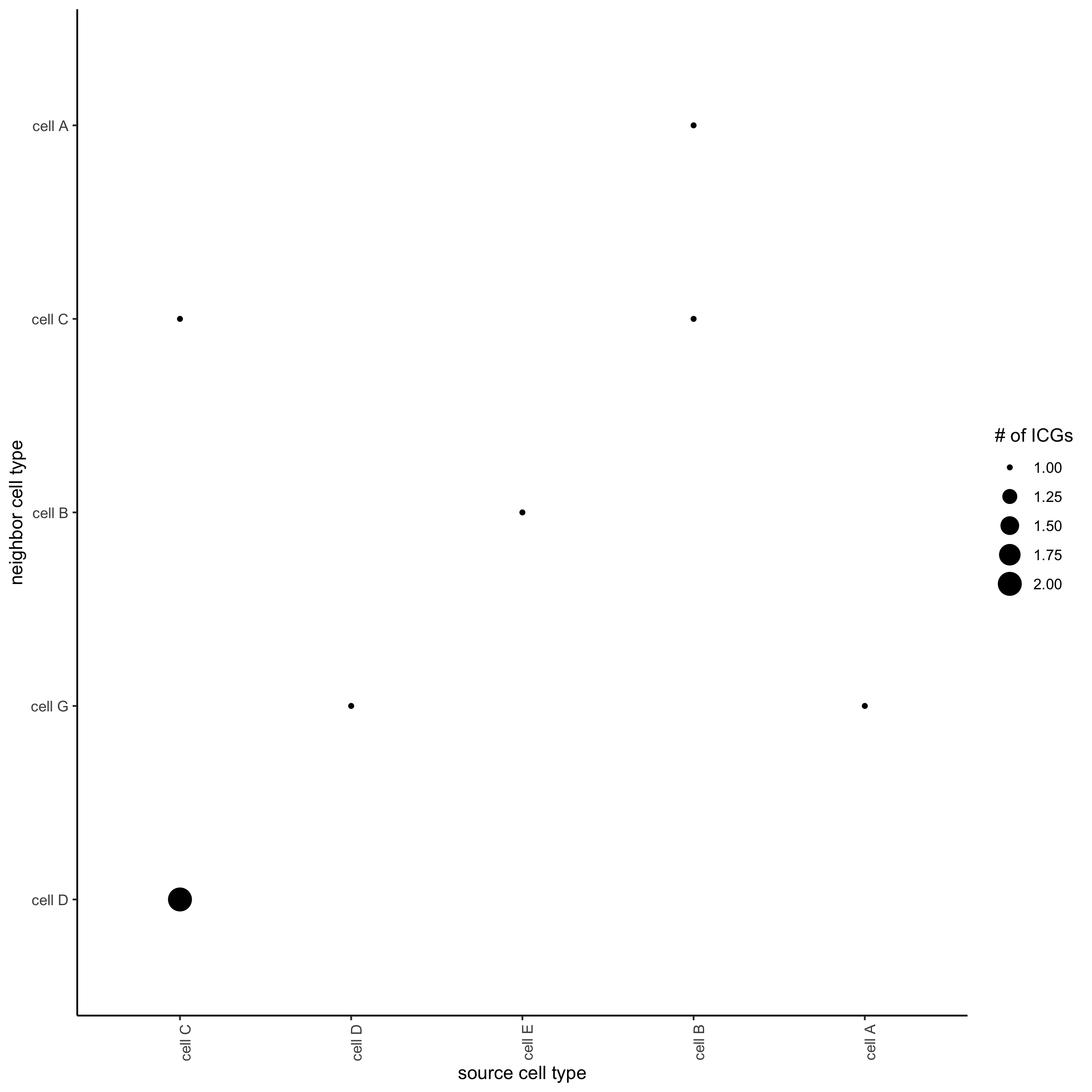
## filter genes
ICGscoresFilt = filterICG(ICGscoresHighGenes,
                          min_cells = 2, min_int_cells = 2, min_fdr = 0.1,
                          min_spat_diff = 0.1, min_log2_fc = 0.1, min_zscore = 1)

## visualize subset of interaction changed genes (ICGs)
ICG_genes = c('Cpne2', 'Scg3', 'Cmtm3', 'Cplx1', 'Lingo1')
ICG_genes_types = c('cell E', 'cell D', 'cell D', 'cell G', 'cell E')
names(ICG_genes) = ICG_genes_types

plotICG(gobject = seqfish_mini,
        cpgObject = ICGscoresHighGenes,
        source_type = 'cell A',
        source_markers = c('Csf1r', 'Laptm5'),
        ICG_genes = ICG_genes)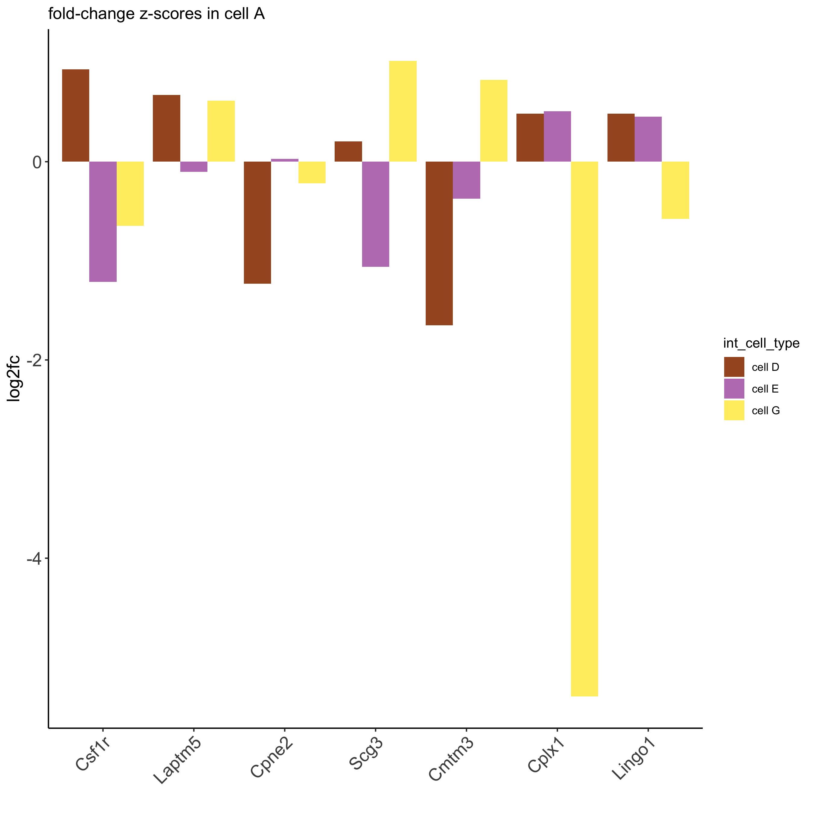
14. cell neighborhood: ligand-receptor cell-cell communication
LR_data = data.table::fread(system.file("extdata", "mouse_ligand_receptors.txt", package = 'Giotto'))

LR_data[, ligand_det := ifelse(mouseLigand %in% seqfish_mini@gene_ID, T, F)]
LR_data[, receptor_det := ifelse(mouseReceptor %in% seqfish_mini@gene_ID, T, F)]
LR_data_det = LR_data[ligand_det == T & receptor_det == T]
select_ligands = LR_data_det$mouseLigand
select_receptors = LR_data_det$mouseReceptor


## get statistical significance of gene pair expression changes based on expression ##
expr_only_scores = exprCellCellcom(gobject = seqfish_mini,
                                   cluster_column = 'cell_types',
                                   random_iter = 500,
                                   gene_set_1 = select_ligands,
                                   gene_set_2 = select_receptors)

## get statistical significance of gene pair expression changes upon cell-cell interaction
spatial_all_scores = spatCellCellcom(seqfish_mini,
                                     spatial_network_name = 'Delaunay_network',
                                     cluster_column = 'cell_types',
                                     random_iter = 500,
                                     gene_set_1 = select_ligands,
                                     gene_set_2 = select_receptors,
                                     adjust_method = 'fdr',
                                     do_parallel = T,
                                     cores = 4,
                                     verbose = 'none')


## * plot communication scores ####

## select top LR ##
selected_spat = spatial_all_scores[p.adj <= 0.5 & abs(log2fc) > 0.1 & lig_nr >= 2 & rec_nr >= 2]
data.table::setorder(selected_spat, -PI)

top_LR_ints = unique(selected_spat[order(-abs(PI))]$LR_comb)[1:33]
top_LR_cell_ints = unique(selected_spat[order(-abs(PI))]$LR_cell_comb)[1:33]

plotCCcomHeatmap(gobject = seqfish_mini,
                 comScores = spatial_all_scores,
                 selected_LR = top_LR_ints,
                 selected_cell_LR = top_LR_cell_ints,
                 show = 'LR_expr')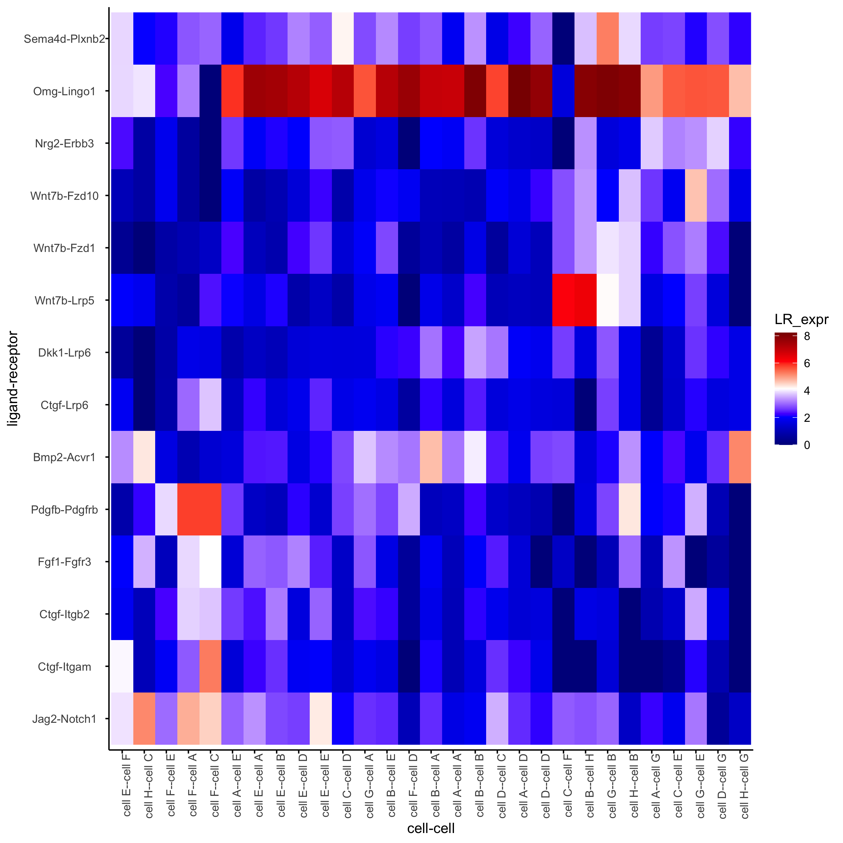
plotCCcomDotplot(gobject = seqfish_mini,
                 comScores = spatial_all_scores,
                 selected_LR = top_LR_ints,
                 selected_cell_LR = top_LR_cell_ints,
                 cluster_on = 'PI')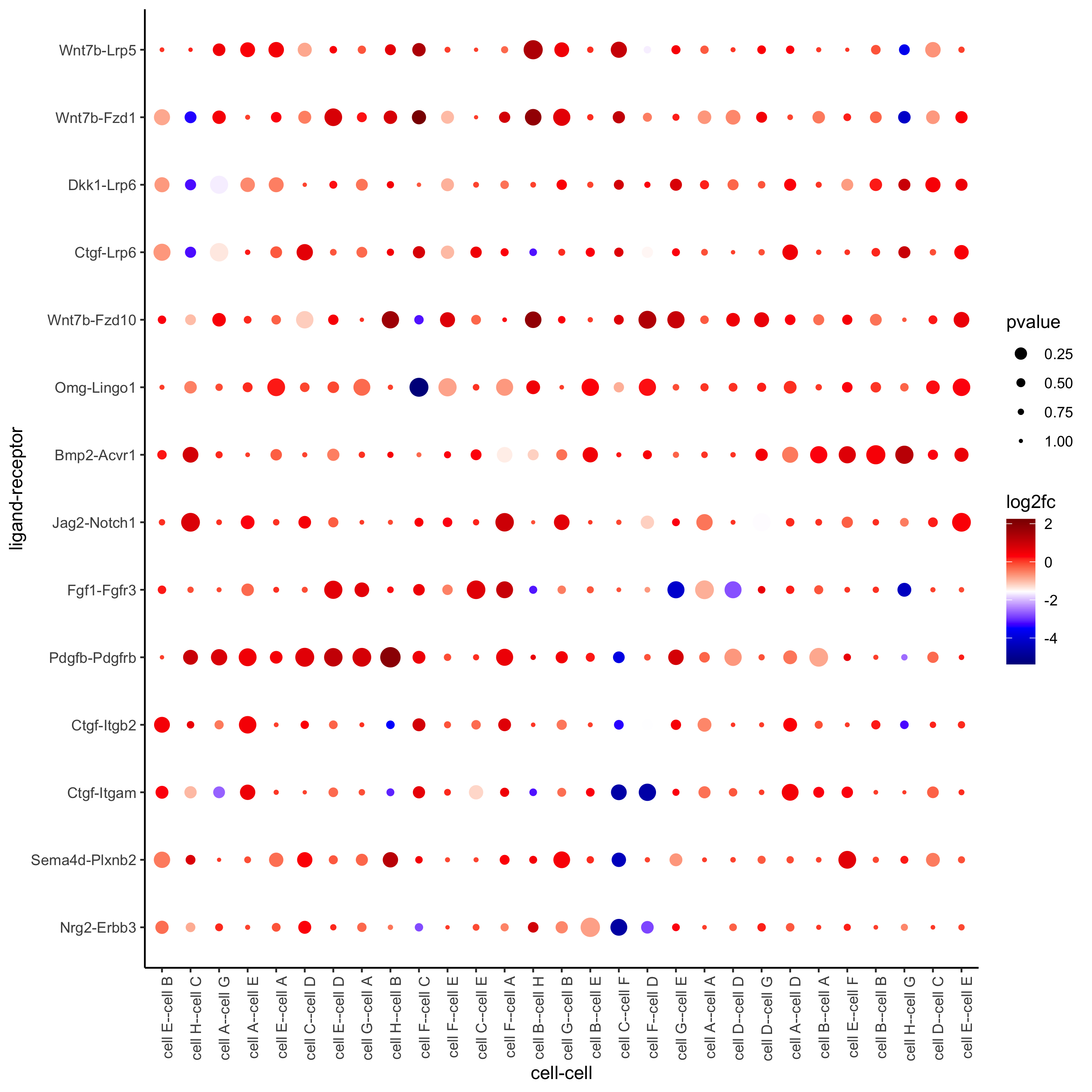
## * spatial vs rank ####
comb_comm = combCCcom(spatialCC = spatial_all_scores,
                      exprCC = expr_only_scores)

# top differential activity levels for ligand receptor pairs
plotRankSpatvsExpr(gobject = seqfish_mini,
                   comb_comm,
                   expr_rnk_column = 'exprPI_rnk',
                   spat_rnk_column = 'spatPI_rnk',
                   midpoint = 10)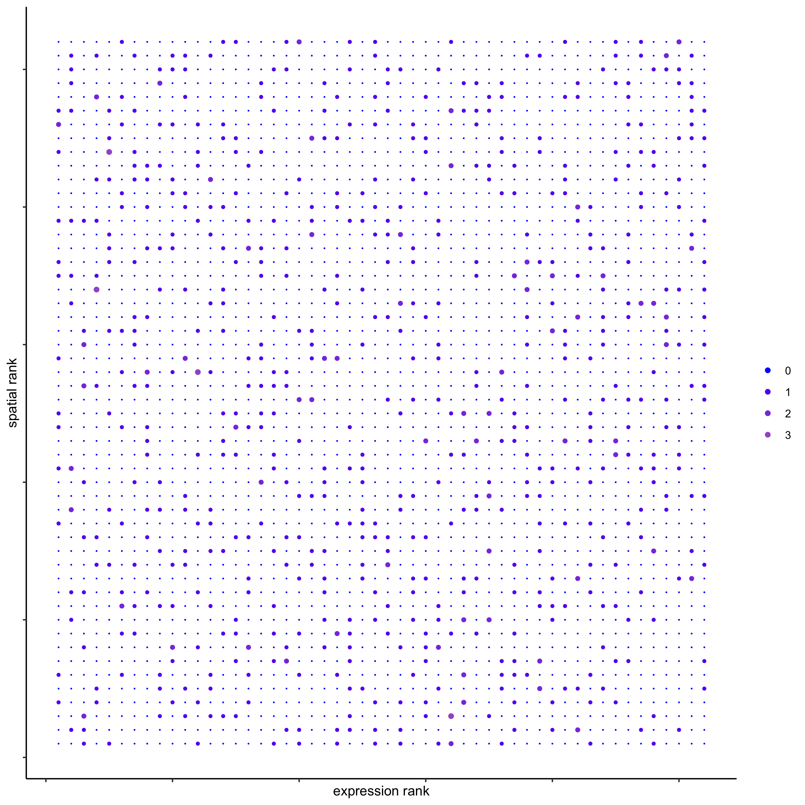
## * recovery ####
## predict maximum differential activity
plotRecovery(gobject = seqfish_mini,
             comb_comm,
             expr_rnk_column = 'exprPI_rnk',
             spat_rnk_column = 'spatPI_rnk',
             ground_truth = 'spatial')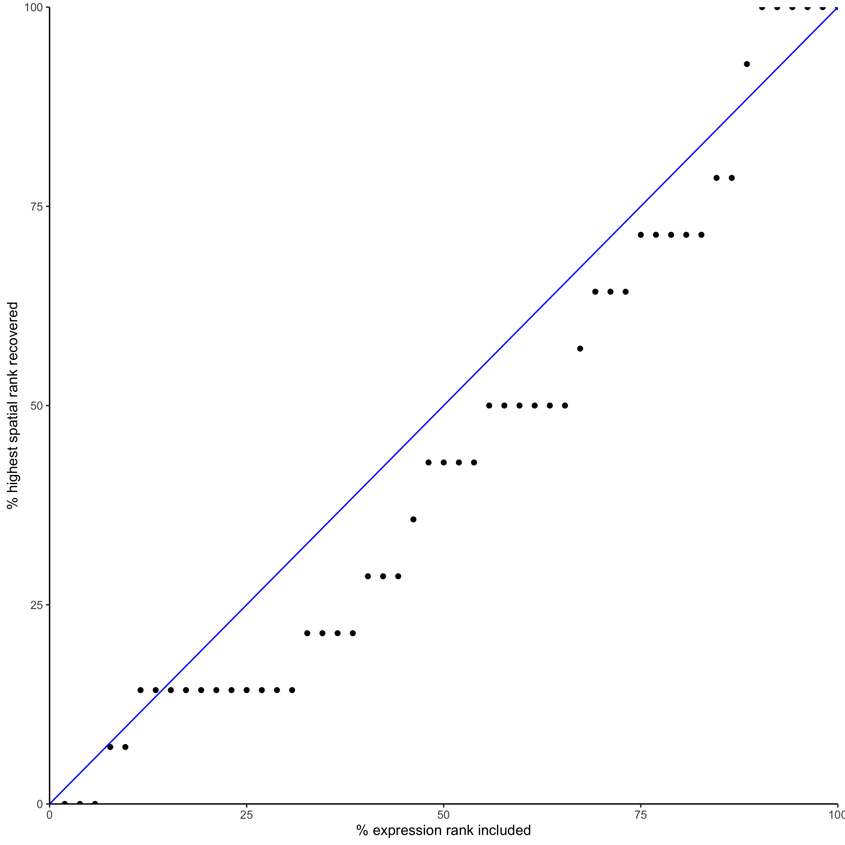
15. export Giotto Analyzer to Viewer
viewer_folder = paste0(temp_dir, '/', 'Mouse_cortex_viewer')

# select annotations, reductions and expression values to view in Giotto Viewer
exportGiottoViewer(gobject = seqfish_mini, output_directory = viewer_folder,
                   factor_annotations = c('cell_types',
                                          'leiden_clus',
                                          'HMRF_k9_b.28'),
                   numeric_annotations = 'total_expr',
                   dim_reductions = c('umap'),
                   dim_reduction_names = c('umap'),
                   expression_values = 'scaled',
                   expression_rounding = 3,
                   overwrite_dir = T)